MODULE LLSQ_Procedures¶

Module LLSQ_Procedures exports routines for solving linear least squares problems and related computations [Golub_VanLoan:1996] [Lawson_Hanson:1974] [Hansen_etal:2012].

More precisely, routines provided in the LLSQ_Procedures module compute solution of the problem

$\min_x || b - MAT * x ||_2$

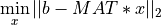
where MAT is a m-by-n real matrix, b is a m-element vector and x a n-element vector and $|| ||_2$ is the 2-norm, or of the problem

$\min_X || B - MAT * X ||_F$

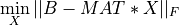
where MAT, B and X are m-by-n, m-by-p and n-by-p real matrices, respectively, and $|| ||_F$ is the Frobenius norm.

These linear least squares solvers are based on the QR decomposition, the QR decomposition with Column Pivoting (QRCP), the Complete Orthogonal Decomposition (COD) and the Singular Value Decomposition (SVD) provided by the QR_Procedures and SVD_Procedures modules. In addition, randomized versions of the QRCP and COD [Duersch_Gu:2017] [Martinsson_etal:2017] [Duersch_Gu:2020] [Martinsson:2019], which are available in module Random and are much faster than their deterministic counterparts, can also be used to solve the above two problems.

Assuming for simplicity that m>=n and MAT has full column rank, the QR decomposition of MAT is

$MAT = Q * R$

and the solution of the (first) linear least square problem in that case is

$x = R^{-1} * [Q^T * b](:n)$

Assuming now that m>=n, but MAT has deficient column rank with $r = {\rm rank}$ (MAT), the QRCP of MAT is

$MAT*P \simeq Q * \left[ \begin{matrix} R11 & R12 \\ 0 & 0 \end{matrix} \right]$

where P is a permutation of the columns of I_n, the identity matrix of order n, R11 is a r-by-r full rank upper triangular matrix and R12 is a r-by-(n-r) matrix. Using this QRCP decomposition, the so-called basic solution of the (first) linear least square problem is now

$x = P * \left( \begin{matrix} R11^{-1} * [Q^T * b](:r) \\ 0 \end{matrix} \right)$

This solution has at least n-r zero components, which corresponds to using only the first r columns of MAT*P in the solution. Interestingly, this implies that the vector b can be approximated by the smallest subset of r columns of MAT. Note, however, that in this case the solution of the linear least square problem is not unique [Lawson_Hanson:1974] [Golub_VanLoan:1996] [Hansen_etal:2012] and it can be demonstrated that the general solution is now given by

$x^* = P * \left( \begin{matrix} R11^{-1} * ( [Q^T * b](:r) - R12 * y) \\ y \end{matrix} \right)$

where y is an arbitrary (n-r)-element vector [Hansen_etal:2012].

Assuming now that MAT is a deficient matrix with $r = {\rm rank}(MAT)$ , the COD of MAT allows us to compute the unique minimum 2-norm solution of our linear least square problem as

$x = P * Z^T \left( \begin{matrix} T11^{-1} * [Q^T * b](:r) \\ 0 \end{matrix} \right)$

with the COD defined as

$MAT * P = Q * \left[ \begin{matrix} T11 & 0 \\ 0 & 0 \end{matrix} \right] * Z$

where T11 is a r-by-r upper triangular full rank matrix and Z is a n-by-n orthogonal matrix. See the manual of the QR_Procedures module for more details.

Finally, the SVD of MAT (which is a special case of the COD described above in which P is the identity matrix and T11 is a diagonal matrix) allows to compute the generalized inverse of MAT, $MAT^+$ , by setting to zero the smallest singular values of MAT, which are below a suitable threshold selected to estimate accurately the rank of MAT [Lawson_Hanson:1974] [Golub_VanLoan:1996] [Hansen_etal:2012]. Using such generalized inverse, the minimum 2-norm solution of our linear least square problem is given by

$x = MAT^+ * b$

See the llsq_svd_solve() or llsq_svd_solve() subroutines for more details on using the SVD for solving linear least square problems with maximum accuracy.

Please note that routines provided in this module apply only to real data of kind stnd. The real kind type stnd is defined in module Select_Parameters.

In order to use one of these routines, you must include an appropriate use LLSQ_Procedures or use Statpack statement in your Fortran program, like:

use LLSQ_Procedures, only: solve_llsq

or :

use Statpack, only: solve_llsq

Here is the list of the public routines exported by module LLSQ_Procedures:

solve_llsq()¶

Purpose:

solve_llsq() computes a solution to a real linear least squares problem:

$\min_X || B - A * X ||_2$

using a QRCP or COD factorization of A. A is a m-by-n matrix which may be rank-deficient. m>=n or n>m is permitted.

B is a right hand side vector (or matrix), and X is a solution vector (or matrix).

The function returns the solution vector or matrix X. In case of a rank deficient matrix A, the minimum 2-norm solution can be computed at the user option (e.g., by using the optional logical argument MIN_NORM with the value true).

Input arguments A and B are not overwritten by solve_llsq().

Synopsis:

x(:n)     = solve_llsq( a(:m,:n) , b(:m)     , krank=krank , tol=tol , min_norm=min_norm )
x(:n,:nb) = solve_llsq( a(:m,:n) , b(:m,:nb) , krank=krank , tol=tol , min_norm=min_norm )
x         = solve_llsq( a(:m)    , b(:m)     )
x(:nb)    = solve_llsq( a(:m)    , b(:m,:nb) )

Examples:

ex1_solve_llsq.F90

ex2_solve_llsq.F90

llsq_qr_solve()¶

Purpose:

llsq_qr_solve() computes a solution to a real linear least squares problem:

$\min_X || B - MAT * X ||_2$ or $\min_X || B - VEC * X ||_2$

using a QRCP or COD factorization of MAT. Here MAT is a m-by-n matrix, which may be rank-deficient, m>=n or n>m is permitted, and VEC is a m-vector.

B is a right hand side vector (or matrix), and X is a solution vector (or matrix).

This subroutine computes the solution vector or matrix X as function solve_llsq() described above and, optionally, the rank of MAT, the residual vector (or matrix) of the linear least squares problem or its 2-norm. In case of a rank deficient matrix MAT, the minimum 2-norm solution can be computed at the user option (e.g., by using the optional logical argument MIN_NORM with the value true).

Input arguments MAT, VEC and B are not overwritten by llsq_qr_solve().

Synopsis:

call llsq_qr_solve( mat(:m,:n) , b(:m)     , x(:n)     , rnorm=rnorm      , resid=resid(:m)     , krank=krank , tol=tol , min_norm=min_norm )
call llsq_qr_solve( mat(:m,:n) , b(:m,:nb) , x(:n,:nb) , rnorm=rnorm(:nb) , resid=resid(:m,:nb) , krank=krank , tol=tol , min_norm=min_norm )
call llsq_qr_solve( vec(:m)    , b(:m)     , x         , rnorm=rnorm      , resid=resid(:m)     )
call llsq_qr_solve( vec(:m)    , b(:m,:nb) , x(:nb)    , rnorm=rnorm(:nb) , resid=resid(:m,:nb) )

Examples:

ex1_llsq_qr_solve.F90

ex2_llsq_qr_solve.F90

ex3_llsq_qr_solve.F90

llsq_qr_solve2()¶

Purpose:

llsq_qr_solve2() computes a solution to a real linear least squares problem:

$\min_X || B - MAT * X ||_2$ or $\min_X || B - VEC * X ||_2$

using a QRCP or COD factorization of MAT. Here MAT is a m-by-n matrix, which may be rank-deficient, m>=n or n>m is permitted, and VEC is a m-vector.

B is a right hand side vector (or matrix) and X is a solution vector (or matrix).

The subroutine computes the solution vector or matrix X and, optionally, the rank of MAT, the residual vector of the linear least squares problem or its 2-norm. In case of a rank deficient matrix MAT, the minimum 2-norm solution can be computed at the user option (e.g., by using the optional logical argument MIN_NORM with the value true).

Arguments MAT, VEC and B are overwritten with information generated by llsq_qr_solve2(). This is the main difference between llsq_qr_solve2() and subroutine llsq_qr_solve() described above.

A second difference with llsq_qr_solve() is that the QRCP or COD decompositions of MAT can be saved in arguments MAT, DIAGR, BETA, IP and TAU on exit at the user option and reused later for solving linear least squares problems with other right hand side vectors or matrices.

Synopsis:

call llsq_qr_solve2( mat(:m,:n) , b(:m)     , x(:n)     , rnorm=rnorm      , comp_resid=comp_resid , krank=krank , tol=tol , min_norm=min_norm , diagr=diagr(:min(m,n)) , beta=beta(:min(m,n)) , ip=ip(:n) , tau=tau(:min(m,n)) )
call llsq_qr_solve2( mat(:m,:n) , b(:m,:nb) , x(:n,:nb) , rnorm=rnorm(:nb) , comp_resid=comp_resid , krank=krank , tol=tol , min_norm=min_norm , diagr=diagr(:min(m,n)) , beta=beta(:min(m,n)) , ip=ip(:n) , tau=tau(:min(m,n)) )
call llsq_qr_solve2( vec(:m)    , b(:m)     , x         , rnorm=rnorm      , comp_resid=comp_resid , diagr=diagr , beta=beta )
call llsq_qr_solve2( vec(:m)    , b(:m,:nb) , x(:nb)    , rnorm=rnorm(:nb) , comp_resid=comp_resid , diagr=diagr , beta=beta )

Examples:

ex1_llsq_qr_solve2.F90

ex2_llsq_qr_solve2.F90

ex3_llsq_qr_solve2.F90

qr_solve()¶

Purpose:

qr_solve() solves overdetermined or underdetermined real linear systems

$MAT * X = B$

with a m-by-n matrix MAT, using a QR factorization of MAT as computed by qr_cmp() in module QR_Procedures. m>=n or n>m is permitted, but it is assumed that MAT has full rank.

B is a right hand side vector (or matrix) and X is a solution vector (or matrix).

It is assumed that qr_cmp() has been used to compute the QR factorization of MAT before calling qr_solve(). The input arguments MAT, DIAGR and BETA of qr_solve() give the QR factorization of MAT and assume the same formats as used for the corresponding output arguments of qr_cmp().

Synopsis:

call qr_solve( mat(:m,:n) , diagr(:min(m,n)) , beta(:min(m,n)) , b(:m)     , x(:n)     , rnorm=rnorm      , comp_resid=comp_resid )
call qr_solve( mat(:m,:n) , diagr(:min(m,n)) , beta(:min(m,n)) , b(:m,:nb) , x(:n,:nb) , rnorm=rnorm(:nb) , comp_resid=comp_resid )

Examples:

ex1_qr_solve.F90

ex2_qr_cmp.F90

qr_solve2()¶

Purpose:

qr_solve2() solves overdetermined or underdetermined real linear systems

$MAT * X = B$

with a m-by-n matrix MAT, using a QRCP or COD decomposition of MAT as computed by subroutines qr_cmp2() or partial_qr_cmp() in module QR_Procedures or subroutines partial_rqr_cmp() and partial_rqr_cmp2() in module Random. m>=n or n>m is permitted and MAT may be rank-deficient.

B is a right hand side vector (or matrix) and X is a solution vector (or matrix).

In case of a rank deficient matrix MAT and a COD of MAT is used in input of qr_solve2(), the minimum 2-norm solution is computed.

It is assumed that qr_cmp2(), partial_qr_cmp(), partial_rqr_cmp() or partial_rqr_cmp2() have been used to compute the QRCP or COD of MAT before calling qr_solve2().

The input arguments MAT, DIAGR, BETA, IP and TAU give the QRCP or COD of MAT and assume the same formats as used for the corresponding output arguments of qr_cmp2(), partial_qr_cmp(), partial_rqr_cmp() or partial_rqr_cmp2().

Synopsis:

call qr_solve2( mat(:m,:n) , diagr(:min(m,n)) , beta(:min(m,n)) , ip(:n) , krank , b(:m)     , x(:n)     , rnorm=rnorm      , comp_resid=comp_resid , tau=tau(:min(m,n)) )
call qr_solve2( mat(:m,:n) , diagr(:min(m,n)) , beta(:min(m,n)) , ip(:n) , krank , b(:m,:nb) , x(:n,:nb) , rnorm=rnorm(:nb) , comp_resid=comp_resid , tau=tau(:min(m,n)) )

Examples:

ex1_qr_solve2.F90

ex2_qr_cmp2.F90

ex3_qr_cmp2.F90

ex3_partial_qr_cmp.F90

ex3_partial_rqr_cmp.F90

ex3_partial_rqr_cmp2.F90

rqb_solve()¶

Purpose:

rqb_solve() computes approximate solutions to overdetermined or underdetermined real linear systems

$MAT * X = (Q * B) * X = C$

with a m-by-n matrix MAT, using a randomized and approximate QRCP or COD decompositions of MAT as computed by subroutine rqb_cmp() in module Random. m>=n or n>m is permitted and MAT may be rank-deficient.

Here C is a right hand side vector (or matrix), X is an approximate solution vector (or matrix), Q is a m-by-nqb matrix with orthonormal columns and B is a nqb-by-n upper trapezoidal matrix as computed by rqb_cmp() with logical argument COMP_QR equals to true or with optional arguments IP and/or TAU present.

It is assumed that rqb_cmp() has been used to compute the randomized and approximate QRCP or COD of MAT before calling rqb_solve().

The input arguments Q, B, IP and TAU give the randomized and approximate QRCP or COD of MAT and assume the same formats as used for the corresponding output arguments of rqb_cmp().

Synopsis:

call rqb_solve( q(:m,:nqb) , b(:nqb,:n) , c(:m) ,     x(:n) ,     ip=ip(:n) , tau=tau(:nqb) , comp_resid=comp_resid )
call rqb_solve( q(:m,:nqb) , b(:nqb,:n) , c(:m,:nc) , x(:n,:nc) , ip=ip(:n) , tau=tau(:nqb) , comp_resid=comp_resid )

Examples:

ex1_rqb_solve.F90

llsq_svd_solve()¶

Purpose:

llsq_svd_solve() computes the minimum 2-norm solution to a real linear least squares problem:

$\min_X || B - MAT * X ||_2$

using the SVD of MAT. MAT is a m-by-n matrix which may be rank-deficient. A cache-efficient blocked and parallel version of the classic Golub and Kahan Householder bidiagonalization [Golub_VanLoan:1996] [Reinsch_Richter:2023], which reduces the traffic on the data bus from four reads and two writes per column-row elimination of the bidiagonalization process to one read and one write [Howell_etal:2008], is used in the first phase of the SVD algorithm.

Several right hand side vectors b and solution vectors x can be handled in a single call; they are stored as the columns of the m-by-nrhs right hand side matrix B and the n-by-nrhs solution matrix X, respectively.

The practical rank of MAT, krank, is determined by treating as zero those singular values which are less than TOL times the largest singular value.

Synopsis:

call llsq_svd_solve( mat(:m,:n) , b(:m)     , failure , x(:n)     , singvalues=singvalues(:min(m,n)) , krank=krank , rnorm=rnorm      , tol=tol ,  mul_size=mul_size , maxiter=maxiter , max_francis_steps=max_francis_steps , perfect_shift=perfect_shift , bisect=bisect , dqds=dqds )
call llsq_svd_solve( mat(:m,:n) , b(:m,:nb) , failure , x(:n,:nb) , singvalues=singvalues(:min(m,n)) , krank=krank , rnorm=rnorm(:nb) , tol=tol ,  mul_size=mul_size , maxiter=maxiter , max_francis_steps=max_francis_steps , perfect_shift=perfect_shift , bisect=bisect , dqds=dqds )

Examples:

ex1_llsq_svd_solve.F90

ex2_llsq_svd_solve.F90

llsq_svd_solve2()¶

Purpose:

llsq_svd_solve2() computes the minimum 2-norm solution to a real linear least squares problem:

$\min_X || B - MAT * X ||_2$

using the SVD of MAT. MAT is a m-by-n with m>=:data:n matrix which may be rank-deficient. A blocked (e.g., “BLAS3”) and parallel version of the one-sided Ralha-Barlow bidiagonal reduction algorithm [Ralha:2003] [Barlow_etal:2005] [Bosner_Barlow:2007] is used in the first phase of the SVD algorithm.

Several right hand side vectors b and solution vectors x can be handled in a single call; they are stored as the columns of the m-by-nrhs right hand side matrix B and the n-by-nrhs solution matrix X, respectively.

The practical rank of MAT, krank, is determined by treating as zero those singular values which are less than TOL times the largest singular value.

In serial or parallel modes (e.g., when OpenMP is used) with a reduced number of processors, llsq_svd_solve2() can be significantly faster than llsq_svd_solve(). However, in parallel mode, but with a large number of processors, llsq_svd_solve() is likely to be faster then llsq_svd_solve2().

Synopsis:

call llsq_svd_solve2( mat(:m,:n) , b(:m)     , failure , x(:n)     , singvalues=singvalues(:min(m,n)) , krank=krank , rnorm=rnorm      , tol=tol ,  mul_size=mul_size , maxiter=maxiter , max_francis_steps=max_francis_steps , perfect_shift=perfect_shift , bisect=bisect , dqds=dqds )
call llsq_svd_solve2( mat(:m,:n) , b(:m,:nb) , failure , x(:n,:nb) , singvalues=singvalues(:min(m,n)) , krank=krank , rnorm=rnorm(:nb) , tol=tol ,  mul_size=mul_size , maxiter=maxiter , max_francis_steps=max_francis_steps , perfect_shift=perfect_shift , bisect=bisect , dqds=dqds )

Examples:

ex1_llsq_svd_solve2.F90

Previous topic

Next topic

MODULE LLSQ_Procedures¶