MODULE SVD_Procedures¶

Module SVD_Procedures exports a large set of routines for computing the full or partial Singular Value Decomposition (SVD), the full or partial QLP Decomposition and the generalized inverse of a matrix and related computations (e.g., bidiagonal reduction of a general matrix, bidiagonal SVD solvers, …) [Lawson_Hanson:1974] [Golub_VanLoan:1996] [Stewart:1999b] [Reinsch_Richter:2023].

Fast methods for obtaining approximations of a truncated SVD or QLP decomposition of rectangular matrices or EigenValue Decomposition (EVD) of symmetric positive semi-definite matrices based on randomization algorithms are also included [Halko_etal:2011] [Martinsson:2019] [Xiao_etal:2017] [Feng_etal:2019] [Duersch_Gu:2020] [Wu_Xiang:2020].

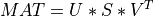
A general rectangular m-by-n matrix MAT has a SVD into the product of a m-by-min(m,n) orthogonal matrix U (e.g., $U^T * U = I$ ), a min(m,n)-by-min(m,n) diagonal matrix of singular values S and the transpose of a n-by-min(m,n) orthogonal matrix V (e.g., $V^T * V = I$ ),

$MAT = U * S * V^T$

The singular values $S(i,i)=\sigma_i$ are all non-negative and can be chosen to form a non-increasing sequence,

$\sigma_1 \ge \sigma_2 \ge ... \ge \sigma_{min(m,n)} \ge 0$

Note that the driver routines in the SVD_Procedures module compute the thin version of the SVD with U and V as m-by-min(m,n) and n-by-min(m,n) matrices with orthonormal columns, respectively. This reduces the needed workspace or allows in-place computations and is the most commonly-used SVD form in practice.

Mathematically, the full SVD is defined with U as a m-by-m orthogonal matrix, V a a n-by-n orthogonal matrix and S as a m-by-n diagonal matrix (with additional rows or columns of zeros). This full SVD can also be computed with the help of the computational routines included in the SVD_Procedures module at the user option.

The SVD of a matrix has many practical uses [Lawson_Hanson:1974] [Golub_VanLoan:1996] [Hansen_etal:2012]. The condition number of the matrix (induced by the vector Euclidean norm), if not infinite, is given by the ratio of the largest singular value to the smallest singular value [Golub_VanLoan:1996] and the presence of a zero singular value indicates that the matrix is singular and that this condition number is infinite. The number of non-zero singular values indicates the rank of the matrix. In practice, the SVD of a rank-deficient matrix will not produce exact zeroes for singular values, due to finite numerical precision. Small singular values should be set to zero explicitly by choosing a suitable tolerance and this is the strategy followed for computing the generalized (e.g., Moore-Penrose) inverse MAT⁺ of a matrix or for solving rank-deficient linear least squares problems with the SVD [Golub_VanLoan:1996] [Hansen_etal:2012]. See the documentations of comp_ginv() subroutine in this module or of llsq_svd_solve() and llsq_svd_solve2() subroutines in LLSQ_Procedures module for more details.

For a rank-deficient matrix, the null space of MAT is given by the span of the columns of V corresponding to the zero singular values in the full SVD of MAT. Similarly, the range of MAT is given by the span of the columns of U corresponding to the non-zero singular values.

See [Lawson_Hanson:1974], [Golub_VanLoan:1996] or [Hansen_etal:2012] for more details on these various results related to the SVD of a matrix.

For very large matrices, the classical SVD algorithms are prohibitively computationally expensive. In such cases, the QLP decomposition provides a reasonable and cheap estimate of the SVD of a matrix, especially when this matrix has a low rank or a significant gap in its singular values spectrum [Stewart:1999b] [Huckaby_Chan:2003] [Huckaby_Chan:2005]. The full or partial QLP decomposition has the form:

$MAT \simeq Q * L * P^T$

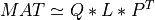
where Q and P are m-by-k and n-by-k matrices with orthonormal columns (and k<=min(m,n)) and L is a k-by-k lower triangular matrix. If k=min(m,n), the QLP factorization is complete and

$MAT = Q * L * P^T$

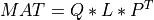
The QLP factorization can be obtained by a two-step algorithm:

in a first step, a partial (or complete) QR factorization with Column Pivoting (QRCP) of MAT is computed;
in a second step, a LQ decomposition of the (eventually row-permuted in decreasing order of magnitude of the rows) upper triangular or trapezoidal (e.g., if n> m) factor, R, of this QR decomposition is computed, giving the final (pivoted) QLP decomposition.

See the manual of the QR_Procedures module for an introduction to the QR, QRCP and LQ factorizations. In many cases, the diagonal elements of L track the singular values (in non-increasing order) of MAT with a reasonable accuracy [Stewart:1999b] [Huckaby_Chan:2003] [Huckaby_Chan:2005]. This property and the fact that the QRCP and LQ factorizations can be interleaved and stopped at any point where there is a gap in the diagonal elements of L make the QLP decomposition a reasonable candidate to determine the rank of a matrix or to obtain a good low-rank approximation of a matrix [Stewart:1999b] [Huckaby_Chan:2003].

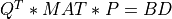
Most of the available SVD algorithms in STATPACK and elsewhere split also in two parts. The first part is a reduction of MAT to bidiagonal form BD in order to reduce the overall computational cost. The second part is the computation of the SVD of this bidiagonal matrix BD, which can be accomplished by several different methods [Golub_VanLoan:1996] [Dongarra_etal:2018].

Thus, as intermediate steps for computing the SVD or for obtaining an accurate partial SVD at a reduced cost, this module also provides routines for

the transformation of MAT to bidiagonal form BD by similarity transformations [Lawson_Hanson:1974] [Golub_VanLoan:1996] [Dongarra_etal:2018],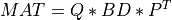

$MAT = Q * BD * P^T$

where Q and P are orthogonal matrices and BD is a min(m,n)-by-min(m,n) upper or lower bidiagonal matrix (e.g., with non-zero entries only on the diagonal and superdiagonal or on the diagonal and subdiagonal). The shape of Q is m-by-min(m,n) and the shape of P is n-by-min(m,n).
the computation of the singular values $\sigma_i$ , left singular vectors $w_i$ and right singular vectors $z_i$ of BD,

$W^T * BD * Z = S$

where S is a min(m,n)-by-min(m,n) diagonal matrix with $S(i,i)=\sigma_i$ , W is the min(m,n)-by-min(m,n) matrix of left singular vectors of BD and Z is the min(m,n)-by-min(m,n) matrix of right singular vectors of BD stored column-wise;
the back-transformation of the singular vectors $w_i$ and $z_i$ of BD to the singular vectors $u_i$ and $v_i$ of MAT [Golub_VanLoan:1996] [Dongarra_etal:2018],

$MAT = (Q * W) * S * (P * Z)^T = U * S * V^T$

where U is the m-by-min(m,n) matrix of the left singular vectors of MAT, V is the n-by-min(m,n) matrix of the right singular vectors of MAT (both stored column-wise) and the singular values $S(i,i)=\sigma_i$ of BD are also the singular values of MAT.

Depending on the situation and the algorithm used, it is also possible to compute only the largest singular values and associated singular vectors of BD and, finally those of MAT.

In what follows, we give some important details about algorithms used in STATPACK for these different intermediate steps: reduction to bidiagonal form BD, computation of the singular values and vectors of BD and back-transformation of the singular vectors of BD to those of MAT.

First, STATPACK includes two different algorithms for the reduction of a matrix to bidiagonal form:

a cache-efficient blocked and parallel version of the classic Golub and Kahan Householder bidiagonalization [Golub_VanLoan:1996] [Reinsch_Richter:2023], which reduces the traffic on the data bus from four reads and two writes per column-row elimination of the bidiagonalization process to one read and one write [Howell_etal:2008];
a blocked (e.g., “BLAS3”) and parallel version of the one-sided Ralha-Barlow bidiagonal reduction algorithm [Ralha:2003] [Barlow_etal:2005] [Bosner_Barlow:2007] , with an eventual partial reorthogonalization based on Gram-Schmidt orthogonalization [Stewart:2007]. This algorithm requires that m>=n and when m<n it is applied to MAT^T instead. In serial mode (e.g., without OpenMP), it is significantly faster in most cases than the first one as the input matrix is only accessed column-wise (e.g., it is an one-sided algorithm), but is less accurate for the left orthonormal vectors stored column-wise in Q as these vectors are computed by a recurrence relationship, which can result in a loss of orthogonality for some matrices with a large condition number [Ralha:2003] [Barlow_etal:2005] [Bosner_Barlow:2007]. A partial reorthogonalization procedure based on Gram-Schmidt orthogonalization [Stewart:2007] has been incorporated into the algorithm in order to correct partially this loss of orthogonality, but is not always sufficient, especially for (large) matrices with a slow decay of singular values near zero. Thus, the loss of orthogonality of Q can be severe for these particular matrices. Fortunately, when the one-sided Ralha-Barlow bidiagonal reduction algorithm is used for computing the SVD of a rectangular matrix, the loss of orthogonality concerns only the left singular vectors associated with the smallest singular values [Barlow_etal:2005]. Furthermore, this deficiency can also be easily corrected a posteriori, if needed, giving fully accurate and fast SVDs for any matrix (see the manuals of the svd_cmp4(), svd_cmp5() and svd_cmp6() SVD drivers in this module, which incorporate such a modification, for details).

The first bidiagonalization reduction algorithm is implemented in bd_cmp() subroutine and the one-sided Ralha-Barlow bidiagonal reduction algorithm is implemented with partial reorthogonalization in bd_cmp2() subroutine and without partial reorthogonalization in bd_cmp3() subroutine. Thus, bd_cmp3() will be significantly faster than bd_cmp2() for low-rank deficient matrices, but a drawback is that Q is not output by bd_cmp3() as this matrix will not be numerically orthogonal in some difficult cases. Among the eight general SVD drivers available in STATPACK:

svd_cmp(), svd_cmp2() and svd_cmp7() use bd_cmp() subroutine for the reduction to bidiagonal form of a rectangular matrix;
svd_cmp3() and svd_cmp8() use bd_cmp2(), e.g., the one-sided Ralha-Barlow bidiagonal reduction algorithm with partial reorthogonalization for this task;
and, finally, svd_cmp4(), svd_cmp5() and svd_cmp6() use bd_cmp3(), e.g., the one-sided Ralha-Barlow bidiagonal reduction algorithm without partial reorthogonalization and a final additional step is required in these SVD drivers to recover all the factors in the SVD of a rectangular matrix.

As a general rule, in a parallel setting (e.g., when OpenMP is used), keep also in mind that the SVD drivers using the bd_cmp() subroutine for the reduction to bidiagonal form will be faster if the number of processors available for the computations is large (e.g., greater than 24 or so), as the number of required synchronization barriers is small in bd_cmp() subroutine. On the other hand, if the number of available processors is small (e.g., less than 16 or so), the SVD drivers using the bd_cmp2() or bd_cmp3() bidiagonal reduction subroutines will be generally faster because these routines use blocked (e.g., “BLAS3”) algorithms; but the number of required synchronization barriers is larger in these two routines, which explains why their performance is degraded compared to bd_cmp() when many processors are available.

Blocked (e.g., “BLAS3”) and parallel routines are also provided for generation and application of the orthogonal matrices, Q and P associated with the bidiagonalization process in both cases [Dongarra_etal:1989] [Golub_VanLoan:1996] [Walker:1988]. See the manuals of ortho_gen_bd(), ortho_gen_bd2(), ortho_gen_q_bd() and ortho_gen_p_bd() subroutines for details.

STATPACK also includes several different algorithms for computing all or selected singular values of a bidiagonal matrix BD:

bidiagonal QR iteration with implicit (Wilkinson) shift [Lawson_Hanson:1974] [Golub_VanLoan:1996] [Reinsch_Richter:2023] ;
bisection applied to the Tridiagonal Golub-Kahan (TGK) form of a bidiagonal matrix or implicitly to the associated symmetric tridiagonal matrix BD^T * BD [Golub_VanLoan:1996] [Fernando:1998] ;
and, finally, Differential Quotient Difference with Shifts (DQDS) algorithms [Fernando_Parlett:1994] [Li_etal:2014].

The bidiagonal implicit QR algorithm applies a sequence of similarity transformations to the bidiagonal matrix BD until its off-diagonal elements become negligible and the diagonal elements have converged to the singular values of BD. It consists of a bulge-chasing procedure that implicitly includes shifts and use plane rotations (e.g., Givens rotations) which preserve the bidiagonal form of BD [Lawson_Hanson:1974] [Golub_VanLoan:1996] [Reinsch_Richter:2023]. Bidiagonal QR iteration with implicit shift is implemented in the generic bd_svd() and bd_svd2() subroutines.

Bisection is a standard method for computing eigenvalues or singular values of a matrix [Golub_VanLoan:1996]. Bisection is based on Sturm sequences and requires $O(min(n,m).k)$ or $O(2min(n,m).k)$ operations to compute k singular values of a min(n,m)-by-min(n,m) bidiagonal matrix BD [Golub_VanLoan:1996] [Fernando:1998]. Two parallel bisection algorithms for bidiagonal matrices are currently implemented in STATPACK:

The first applies bisection to an associated 2.min(n,m)-by-2.min(n,m) symmetric tridiagonal matrix T with zeros on the diagonal (the so-called Tridiagonal Golub-Kahan form of BD) whose eigenvalues are the singular values of BD and their negatives [Fernando:1998] [Marques_etal:2020]. This approach is implemented in bd_singval() subroutine;
The second applies bisection implicitly to the associated min(n,m)-by-min(n,m) symmetric tridiagonal matrix BD^T * BD (but without computing this matrix product) whose eigenvalues are the squares of the singular values of BD by using the differential stationary form of the QD algorithm of Rutishauser (see Sec.3.1 of [Fernando:1998]). This approach is implemented in bd_singval2() subroutine.

If high relative accuracy for small singular values is required, the first bisection algorithm based on the Tridiagonal Golub-Kahan (TGK) form of the bidiagonal matrix is the best choice [Fernando:1998]. Importantly, both STATPACK bidiagonal bisection routines (e.g., bd_singval() and bd_singval2()) also allow subset computations of the (largest) singular values of BD.

The DQDS algorithm is mathematically equivalent to the Cholesky LR method with shifts, applied to tridiagonal symmetric matrices [Fernando_Parlett:1994]. The DQDS algorithm has been popular due to its accuracy, speed and numerical stability, and is implemented as subroutine dlasq() in LAPACK [Parlett_Marques:2000] [Li_etal:2014]. The first version of the DQDS algorithm included in STATPACK is adapted from this dlasq() subroutine in LAPACK and also includes the early aggressive deflation strategy proposed by [Nakatsukasa_etal:2012] at the user option. The second version of the DQDS algorithm included in STATPACK uses a different shift strategy proposed in [Yamashita_etal:2013]. This variant is usually much slower than the first, but may be more accurate for some bidiagonal matrices. These two variants of the DQDS algorithm are provided in the bd_lasq1() and bd_dqds() subroutines, respectively.

All these different singular values computational subroutines are available in the SVD_Procedures module.

The bidiagonal QR and DQDS methods always compute all the singular values of the bidiagonal matrix BD. On the other hand, subset computations are possible with the two bisection algorithms. Keep also in mind that with both the bisection and DQDS methods, the singular values can be computed to high relative accuracy, in the absence of denormalization, underflow and overflow, and this property is important if singular vectors need to be computed in a later step by inverse iteration or deflation (see below). Finally, note that the DQDS algorithm is usually much faster than bisection and as fast than QR if all singular values of BD must be computed and despite that the STATPACK bisection algorithms are parallelized when OpenMP is used.

Among the eight general SVD drivers available in STATPACK:

svd_cmp(), svd_cmp2(), svd_cmp3(), svd_cmp4() and svd_cmp5() use the bidiagonal QR iteration with implicit shift method when both all the singular values and vectors of BD are requested and the DQDS algorithm (by default) when only singular values of the input matrix MAT are requested;
svd_cmp6() uses bisection on the TGK form of BD for computing all or the leading singular values of BD (and the input matrix MAT) in all cases;
and, finally, svd_cmp7() and svd_cmp8() compute all the singular values of BD (and the input matrix MAT) by the first variant of the DQDS algorithm (e.g., bd_lasq1()).

Currently, STATPACK also includes three different methods for computing (selected) singular vectors of a bidiagonal matrix BD:

bidiagonal QR iteration with implicit (Wilkinson) shift [Lawson_Hanson:1974] [Golub_VanLoan:1996] [Reinsch_Richter:2023];
inverse iteration on the Tridiagonal Golub-Kahan (TGK) form of a bidiagonal matrix [Godunov_etal:1993] [Ipsen:1997] [Dhillon:1998] [Marques_Vasconcelos:2017] [Marques_etal:2020];
and a novel deflation perfect shift technique applied directly to the bidiagonal matrix BD based on the works of Godunov and coworkers on the deflation for tridiagonal matrices [Godunov_etal:1993] [Fernando:1997] and [Malyshev:2000].

The bidiagonal QR algorithm is considered as very accurate and robust for computing singular values [Demmel_Kahan:1990], but its implementation in current Dense Linear Algebra softwares for computing singular vectors is far from optimal in terms of speed [VanZee_etal:2011] [Dongarra_etal:2018]. To correct this deficiency and get high performance for computing singular vectors by this bidiagonal implicit QR algorithm, several modifications have been introduced in its implementation in STATPACK by:

restructuring the bidiagonal QR iterations with a wave-front algorithm for the accumulation of Givens rotations [VanZee_etal:2011];
the use of a blocked “BLAS3” algorithm to update the singular vectors by these Givens rotations when possible [Lang:1998];
the use of a novel perfect shift strategy in the QR iterations inspired by the works of [Godunov_etal:1993] [Malyshev:2000] and [Fernando:1997], which reduces significantly the number of QR iterations needed for convergence for many matrices;
and, finally, OpenMP parallelization [Demmel_etal:1993].

With all these changes, the bidiagonal QR algorithm becomes competitive with the divide-and-conquer method for computing the full or thin SVD of a matrix [VanZee_etal:2011]. Subroutines bd_svd() and bd_svd2() use this efficient and improved bidiagonal implicit QR algorithm. However, a drawback is that subset computations are not possible with the bidiagonal QR algorithm [Marques_etal:2020]. With this method, it is possible to compute all the singular values or both all the singular values and associated singular vectors.

The bisection-inverse iteration or bisection-deflation methods are the preferred methods if you are only interested in a subset of the singular vectors and values of a bidiagonal matrix BD or a full matrix MAT [Marques_etal:2020].

Once singular values have been obtained by bisection, DQDS or implicit QR iterations in a first step, associated singular vectors can be computed efficiently using:

Fernando’s method and inverse iteration on the TGK form of the bidiagonal matrix BD [Godunov_etal:1993] [Fernando:1997] [Bini_etal:2005] [Marques_Vasconcelos:2017] [Marques_etal:2020]. These singular vectors are then orthogonalized by the modified Gram-Schmidt or QR algorithms if the singular values are not well-separated. A “BLAS3” and parallelized QR algorithm is used for large clusters of singular values for increased efficiency;
a novel technique combining an extension to bidiagonal matrices of Fernando’s approach for computing eigenvectors of tridiagonal matrices with a deflation procedure by Givens rotations originally developed by Godunov and collaborators [Fernando:1997] [Parlett_Dhillon:1997] [Malyshev:2000]. If this deflation technique failed, QR bidiagonal iterations with a perfect shift strategy are used instead as a back-up procedure [Mastronardi_etal:2006]. It is highly recommended to compute the singular values of the bidiagonal matrix BD to high accuracy for the success of the deflation technique, meaning that this approach is less robust than the inverse iteration technique for computing selected singular vectors of a bidiagonal matrix.

If the distance between the singular values of BD is sufficient relative to the norm of BD, then computing the associated singular vectors by inverse iteration or deflation is also a $O(min(n,m).k)$ or $O(2.min(n,m).k)$ process, where k is the number of singular vectors to compute. Thus, when all singular values are well separated and no orthogonalization is needed, the inverse iteration or deflation methods are much faster than than the bidiagonal implicit QR algorithm for computing the singular vectors in the thin SVD of a matrix. Furthermore, as already discussed above, the inverse iteration or deflation methods are the preferred methods if you are only interested in a subset of the singular vectors of the matrix BD or MAT, as subset computations are not possible in the standard implicit QR algorithm.

bd_inviter() and bd_deflate() generic subroutines implement, respectively, the inverse iteration and deflation methods for computing all or selected singular vectors of bidiagonal matrices and bd_inviter2() and bd_deflate2() generic subroutines perform the same tasks, but for full matrices, once these full matrices have been reduced to bidiagonal form and singular values have been computed by bisection or DQDS. Note that these preliminary tasks can be done efficiently with the help of the select_singval_cmp(), select_singval_cmp2(), select_singval_cmp3() and select_singval_cmp4() subroutines also available in this module.

Among the eight general SVD drivers available in STATPACK, svd_cmp6(), svd_cmp7() and svd_cmp8() uses the inverse iteration method for computing all or the leading singular vectors of BD (and the input matrix MAT).

All above algorithms are parallelized with OpenMP [openmp]. Parallelism concerns only the computation of singular vectors in the bidiagonal implicit QR method, but both the computation of the singular values and singular vectors in the bisection-inverse iteration and bisection-deflation methods. Furthermore, the computation of singular vectors in the bidiagonal QR or inverse iteration methods also uses blocked “BLAS3” algorithms when possible for maximum efficiency [Walker:1988] [Lang:1998].

Note finally that the SVD driver and computational routines provided in this module are very different from the corresponding bidiagonal implicit QR iteration and inverse iteration routines provided by LAPACK [Anderson_etal:1999] and are much faster if OpenMP and BLAS supports are activated, but slightly less accurate for the same precision in their default settings for a few cases.

In addition to these standard and deterministic SVD (or QLP) driver and computational routines based on bidiagonal QR, inverse or deflation iterations applied to bidiagonal matrices after a preliminary bidiagonal reduction step, module SVD_Procedures also includes an extensive set of very fast routines based on randomization techniques for solving the same problems with a much better efficiency (but a decreased accuracy).

For a good and general introduction to randomized linear algebra, see [Li_etal:2017], [Martinsson:2019] and [Erichson_etal:2019]. The recent survey [Tropp_Webber:2023], which focuses specifically on modern approaches for computing low-rank approximations of high-dimensional matrices by means of the randomized SVD, randomized subspace iteration, and randomized block Krylov iteration, is also an excellent reference for many of the randomized algorithms included in module SVD_Procedures for obtaining a low-rank approximation of a high-dimensional matrix at a reduced cost. There are two classes of randomized low-rank approximation algorithms, sampling-based and random projection-based algorithms:

Sampling algorithms use randomly selected columns or rows based on sampling probabilities derived from the original matrix in a first step, and a deterministic algorithm, such as SVD or EVD, is performed on the smaller subsampled matrix;
the projection-based algorithms use the concept of random projections to project the high-dimensional space spanned by the columns of the matrix into a low-dimensional subspace, which approximates the dominant subspace of a matrix. The input matrix is then compressed-either explicitly or implicitly-to this subspace, and the reduced matrix is manipulated inexpensively by standard deterministic methods to obtain the desired low-rank factorization in a second step.

The randomized routines included in module SVD_Procedures are projection-based methods. In many cases, this approach beats largely its classical competitors in terms of speed [Halko_etal:2011] [Musco_Musco:2015] [Li_etal:2017] [Tropp_Webber:2023]. Thus, these routines based on recent randomized projection algorithms are much faster than the standard drivers included in module SVD_Procedures or Eig_Procedures for computing a truncated SVD or EVD of a matrix. Yet, such randomized methods are also shown to compute with a very high probability low-rank approximations that are accurate, and are known to perform even better in many practical situations when the singular values of the input matrix decay quickly [Halko_etal:2011] [Gu:2015] [Li_etal:2017] [Tropp_Webber:2023].

More precisely, module SVD_Procedures includes routines based on randomization for computing:

approximations of the largest singular values and associated left and right singular vectors of full general matrices using randomized power, subspace or block Krylov iterations [Halko_etal:2011] [Gu:2015] [Musco_Musco:2015] [Li_etal:2017] [Tropp_Webber:2023] or randomized QRCP and QLP factorizations [Duersch_Gu:2017] [Xiao_etal:2017] [Feng_etal:2019] [Duersch_Gu:2020] in order to extract the dominant subspace of a matrix;
approximations of the largest eigenvalues and associated eigenvectors of full symmetric positive semi-definite matrices using randomized power, subspace or block Krylov iterations or the Nystrom method [Halko_etal:2011] [Musco_Musco:2015] [Li_etal:2017]. The Nystrom method provides more accurate results for positive semi-definite matrices;
and, finally, randomized partial QLP factorizations, which are also much faster than their deterministic counterparts [Wu_Xiang:2020];

Usually, the problem of low-rank matrix approximation falls into two categories:

the fixed-rank problem, where the rank nsvd of the matrix approximation which is sought is given;
the fixed-precision problem, where we seek a partial SVD factorization, rSVD, with a rank as small as possible, such that

$||MAT-rSVD||_F <= eps$

where eps is a given accuracy tolerance.

Module SVD_Procedures includes four (randomized) routines for solving the fixed-rank problem: rqr_svd_cmp(), rsvd_cmp(), rqlp_svd_cmp() and rqlp_svd_cmp2() and three (randomized) routines for solving the fixed-precision problem: rqr_svd_cmp_fixed_precision(), rsvd_cmp_fixed_precision(), rqlp_svd_cmp_fixed_precision().

rqr_svd_cmp() and rqr_svd_cmp_fixed_precision() are based on a (randomized or deterministic) partial QRCP factorization followed by a SVD step [Xiao_etal:2017]. rsvd_cmp() and rsvd_cmp_fixed_precision() are based on randomized power, subspace or block Krylov iterations followed by a SVD step [Musco_Musco:2015] [Li_etal:2017] [Martinsson_Voronin:2016] [Yu_etal:2018] and, finally, rqlp_svd_cmp(), rqlp_svd_cmp2() and rqlp_svd_cmp_fixed_precision() are based on a (randomized or deterministic) partial QLP factorization followed by a SVD step [Duersch_Gu:2017] [Feng_etal:2019] [Duersch_Gu:2020].

The choice between these different subroutines involves tradeoffs between speed and accuracy. For both the fixed-rank and fixed-precision problems, the routines based on a preliminary partial QRCP factorization are the fastest and the less accurate, and those based on a partial QLP factorization are the most accurate, but the slowest. On the other hand, routines based on randomized power, subspace or block Krylov iterations provide intermediate performances both in terms of accuracy and speed in most cases. In this class of methods, routines based on randomized power iteration return accurate approximations for matrices with rapid singular value decay, but algorithms based on randomized block Krylov iteration perform better for matrices with a moderate or slow singular value decay [Tropp_Webber:2023]. Finally, in case of limited storage, algorithms based on subspace iterations are a good compromise [Tropp_Webber:2023]. Keep also in mind, that if you already know the rank of the matrix approximation you are looking for, routines dedicated to solve the fixed-rank problem (.e.g., rqr_svd_cmp(), rsvd_cmp(), rqlp_svd_cmp() and rqlp_svd_cmp2()) are faster and more accurate than their twin routines dedicated to solve the fixed-precision problem.

Module SVD_Procedures also includes a subroutine, reig_pos_cmp(), for computing approximations of the largest eigenvalues and associated eigenvectors of a full n-by-n real symmetric positive semi-definite matrix MAT using a variety of randomized techniques and, also, three subroutines, qlp_cmp(), qlp_cmp2() and rqlp_cmp(), for computing randomized (or deterministic) full or partial QLP factorizations, which can also be used to solve the fixed-rank problem [Stewart:1999b].

All these randomized SVD or QLP algorithms are also parallelized with OpenMP [openmp].

Finally, note that the routines provided in this module apply only to real data of kind stnd. The real kind type stnd is defined in module Select_Parameters. Computation of singular values and vectors for a complex matrix are not provided in this release of STATPACK.

In order to use one of these routines, you must include an appropriate use SVD_Procedures or use Statpack statement in your Fortran program, like:

use SVD_Procedures, only: svd_cmp

or :

use Statpack, only: svd_cmp

Here is the list of the public routines exported by module SVD_Procedures:

bd_cmp()¶

Purpose:

bd_cmp() reduces a general m-by-n matrix MAT to upper or lower bidiagonal form BD by an orthogonal transformation:

$Q^T * MAT * P = BD$

where Q and P are orthogonal matrices. If:

m >= n, BD is upper bidiagonal;
m < n, BD is lower bidiagonal.

bd_cmp() computes BD, Q and P, using an efficient variant of the classic Golub and Kahan Householder bidiagonalization algorithm [Howell_etal:2008].

Optionally, bd_cmp() can also reduce a general m-by-n matrix MAT to upper bidiagonal form BD by a two-step algorithm:

If m >= n, a QR factorization of the real m-by-n matrix MAT is first computed

$MAT = O * R$

where O is orthogonal and R is upper triangular. In a second step, the n-by-n upper triangular matrix R is reduced to upper bidiagonal form BD by an orthogonal transformation:

$Q^T * R * P = BD$

where Q and P are orthogonal and BD is an upper bidiagonal matrix.
If m < n, a LQ factorization of the real m-by-n matrix MAT is first computed

$MAT = L * O$

where O is orthogonal and L is lower triangular. In a second step, the m-by-m lower triangular matrix L is reduced to upper bidiagonal form BD by an orthogonal transformation :

$Q^T * L * P = BD$

where Q and P are orthogonal and BD is an upper bidiagonal matrix.

This two-step reduction algorithm will be more efficient if m is much larger than n or if n is much larger than m.

These two different reduction algorithms of MAT to bidiagonal form BD are also parallelized with OpenMP.

Synopsis:

call bd_cmp( mat(:m,:n) , d(:min(m,n)) , e(:min(m,n)) , tauq(:min(m,n)) , taup(:min(m,n)) )

call bd_cmp( mat(:m,:n) , d(:min(m,n)) , e(:min(m,n)) , tauq(:min(m,n))                   )

call bd_cmp( mat(:m,:n) , d(:min(m,n)) , e(:min(m,n))                                     )

call bd_cmp( mat(:m,:n) , d(:min(m,n)) , e(:min(m,n)) , tauq(:min(m,n)) , taup(:min(m,n)), rlmat(:min(m,n),:min(m,n)) , tauo=tauo(:min(m,n)) )

Examples:

ex1_bd_cmp.F90

ex1_apply_q_bd.F90

ex1_bd_inviter2.F90

ex1_bd_inviter2_bis.F90

ex1_bd_deflate2.F90

ex1_bd_deflate2_bis.F90

bd_cmp2()¶

Purpose:

bd_cmp2() reduces a m-by-n matrix MAT with m >= n to upper bidiagonal form BD by an orthogonal transformation:

$Q^T * MAT * P = BD$

where Q and P are orthogonal matrices.

bd_cmp2() computes BD, Q and P using a parallel (if OpenMP support is activated) and blocked version of the one-sided Ralha-Barlow bidiagonal reduction algorithm [Ralha:2003] [Barlow_etal:2005] [Bosner_Barlow:2007].

A partial reorthogonalization procedure based on Gram-Schmidt orthogonalization [Stewart:2007] has been incorporated to bd_cmp2() in order to correct partially the loss of orthogonality of Q in the one-sided Ralha-Barlow bidiagonal reduction algorithm [Barlow_etal:2005].

bd_cmp2() is more efficient than bd_cmp() as it is an one-sided algorithm, but is less accurate for the computation of the orthogonal matrix Q.

Synopsis:

call bd_cmp2( mat(:m,:n) , d(:n) , e(:n) , p(:n,:n), failure=failure , gen_p=gen_p, reortho=reortho )
call bd_cmp2( mat(:m,:n) , d(:n) , e(:n) ,           failure=failure              , reortho=reortho )

Examples:

ex1_bd_cmp2.F90

ex2_bd_inviter2.F90

ex2_bd_deflate2.F90

bd_cmp3()¶

Purpose:

bd_cmp3() reduces a m-by-n matrix MAT with m >= n to upper bidiagonal form BD by an orthogonal transformation:

$Q^T * MAT * P = BD$

where Q and P are orthogonal.

bd_cmp3() computes BD and P using a parallel (if OpenMP support is activated) and blocked version of the one-sided Ralha-Barlow bidiagonal reduction algorithm [Ralha:2003] [Barlow_etal:2005] [Bosner_Barlow:2007].

bd_cmp3() is faster than bd_cmp2(), if the Q orthogonal matrix is not needed, especially for matrices with a low rank compared to its dimensions as partial reorthogonalization of Q is not performed in bd_cmp3().

Synopsis:

call bd_cmp3( mat(:m,:n) , d(:n) , e(:n) , gen_p=gen_p , failure=failure )

Examples:

ex1_bd_cmp3.F90

ortho_gen_bd()¶

Purpose:

ortho_gen_bd() generates the real orthogonal matrices Q and P determined by bd_cmp() when reducing a m-by-n real matrix MAT to bidiagonal form:

$MAT = Q * BD * P^T$

Q and P are defined as products of elementary reflectors H(i) and G(i), respectively, as computed by bd_cmp() and stored in its array arguments MAT, TAUQ and TAUP.

If m >= n:

$Q = H(1) * H(2) * ... * H(n)$ and ortho_gen_bd() returns the first n columns of Q in MAT;
$P = G(1) * G(2) * ... * G(n-1)$ and ortho_gen_bd() returns P as an n-by-n matrix in P.

If m < n:

$Q = H(1) * H(2) * ... * H(m-1)$ and ortho_gen_bd() returns Q as an m-by-m matrix in MAT(1:m,1:m);
$P = G(1) * G(2) * ... * G(m)$ and ortho_gen_bd() returns the first m columns of P, in P.

The generation of the real orthogonal matrices Q and P is blocked and parallelized with OpenMP [Walker:1988].

Synopsis:

call ortho_gen_bd( mat(:m,:n) , tauq(:min(m,n)) , taup(:min(m,n)) , p(:n,:min(m,n)) )

Examples:

ex1_bd_cmp.F90

ortho_gen_bd2()¶

Purpose:

ortho_gen_bd2() generates the real orthogonal matrices Q and P^T determined by bd_cmp() when reducing a m-by-n real matrix MAT to bidiagonal form:

$MAT = Q * BD * P^T$

Q and P^T are defined as products of elementary reflectors H(i) and G(i), respectively, as computed by bd_cmp() and stored in its array arguments MAT, TAUQ and TAUP.

If m >= n:

$Q = H(1) * H(2) * ... * H(n)$ and ortho_gen_bd2() returns the first n columns of Q in MAT;
$P^T = G(n-1) * ... * G(2) * G(1)$ and ortho_gen_bd2() returns P^T as a n-by-n matrix in Q_PT.

If m < n:

$Q = H(1) * H(2) * ... * H(m-1)$ and ortho_gen_bd2() returns Q as a m-by-m matrix in Q_PT;
$P^T = G(m) * ... * G(2) * G(1)$ and ortho_gen_bd2() returns the first m rows of P^T, in MAT.

The generation of the real orthogonal matrices Q and P^T is blocked and parallelized with OpenMP [Walker:1988].

Synopsis:

call ortho_gen_bd2( mat(:m,:n) , tauq(:min(m,n)) , taup(:min(m,n)) , q_pt(:min(m,n),:min(m,n)) )

ortho_gen_q_bd()¶

Purpose:

ortho_gen_q_bd() generate the real orthogonal matrix Q determined by bd_cmp() when reducing a m-by-n real matrix MAT to bidiagonal form:

$MAT = Q * BD * P^T$

Q is defined as products of elementary reflectors H(i) as computed by bd_cmp() and stored in its array arguments MAT and TAUQ.

If m >= n:

$Q = H(1) * H(2) * ... * H(n)$ and ortho_gen_q_bd() returns the first n columns of Q in MAT;

If m < n:

$Q = H(1) * H(2) * ... * H(m-1)$ and ortho_gen_q_bd() returns Q as a m-by-m matrix in MAT(1:m,1:m);

The generation of the real orthogonal matrix Q is blocked and parallelized with OpenMP [Walker:1988].

Synopsis:

call ortho_gen_q_bd( mat(:m,:n) , tauq(:min(m,n)) )

Examples:

ex1_ortho_gen_q_bd.F90

ortho_gen_p_bd()¶

Purpose:

ortho_gen_p_bd() generate the real orthogonal matrix P determined by bd_cmp() when reducing a m-by-n real matrix MAT to bidiagonal form:

$MAT = Q * BD * P^T$

P is defined as products of elementary reflectors G(i) determined by bd_cmp() and stored in its array arguments MAT and TAUP.

If m >= n:

$P = G(1) * G(2) * ... * G(n-1)$ and ortho_gen_p_bd() returns P as a n-by-n matrix in P.

If m < n:

$P = G(1) * G(2) * ... * G(m)$ and ortho_gen_p_bd() returns the first m columns of P, in P.

The generation of the real orthogonal matrix P is blocked and parallelized with OpenMP [Walker:1988].

Synopsis:

call ortho_gen_p_bd( mat(:m,:n) , taup(:min(m,n)) , p(:n,:min(m,n)) )

Examples:

ex1_ortho_gen_q_bd.F90

apply_q_bd()¶

Purpose:

apply_q_bd() overwrites the general real m-by-n matrix C with:

$Q * C$ if LEFT = true and TRANS = false ;
$Q^T * C$ if LEFT = true and TRANS = true ;
$C * Q$ if LEFT = false and TRANS = false ;
$C * Q^T$ if LEFT = false and TRANS = true .

Here Q is the orthogonal matrix determined by bd_cmp() when reducing a real matrix MAT to bidiagonal form:

$MAT = Q * BD * P^T$

and Q is defined as products of elementary reflectors H(i).

Let nq = m if LEFT = true and nq = n if LEFT = false. Thus, nq is the order of the orthogonal matrix Q that is applied. MAT is assumed to have been a nq-by-k matrix and

$Q = H(1) * H(2) * ... * H(k)$ , if nq >= k;

or

$Q = H(1) * H(2) * ... * H(nq-1)$ , if nq < k.

The application of the real orthogonal matrix Q to the matrix C is blocked and parallelized with OpenMP [Walker:1988].

Synopsis:

call apply_q_bd( mat(:m,:n) , tauq(:min(m,n)) , c(:,:) , left , trans )

Examples:

ex1_apply_q_bd.F90

ex2_bd_singval.F90

ex2_bd_singval2.F90

apply_p_bd()¶

Purpose:

apply_p_bd() overwrites the general real m-by-n matrix C with

$P * C$ if LEFT = true and TRANS = false ;

$P^T * C$ if LEFT = true and TRANS = true ;

$C * P$ if LEFT = false and TRANS = false ;

$C * P^T$ if LEFT = false and TRANS = true .

Here P is the orthogonal matrix determined by bd_cmp() when reducing a real matrix MAT to bidiagonal form:

$MAT = Q * BD * P^T$

and P is defined as products of elementary reflectors G(i).

Let np = m if LEFT = true and np = n if LEFT = false. Thus, np is the order of the orthogonal matrix P that is applied. MAT is assumed to have been a k-by-np matrix and

$P = G(1) * G(2) * ... * G(k)$ , if k < np;

or

$P = G(1) * G(2) * ... * G(np-1)$ , if k >= np.

The application of the real orthogonal matrix P to the matrix C is blocked and parallelized with OpenMP [Walker:1988].

Synopsis:

call apply_p_bd( mat(:m,:n) , taup(:min(m,n)) , c(:,:) , left , trans )

Examples:

ex1_apply_q_bd.F90

ex2_bd_singval.F90

ex2_bd_singval2.F90

bd_svd()¶

Purpose:

bd_svd() computes the Singular Value Decomposition (SVD) of a real n-by-n (upper or lower) bidiagonal matrix B:

$B = Q * S * P^T$

where S is a diagonal matrix with non-negative diagonal elements (the singular values of B), and, Q and P are orthogonal matrices (P^T denotes the transpose of P).

The routine computes S, U * Q, and V * P, for given real input matrices U, V, using the implicit bidiagonal QR method [Lawson_Hanson:1974] [Golub_VanLoan:1996].

Synopsis:

call bd_svd( upper , d(:n) , e(:n) , failure , u(:,:n) , v(:,:n) , sort=sort , maxiter=maxiter , max_francis_steps=max_francis_steps , perfect_shift=perfect_shift , bisect=bisect , dqds=dqds )

call bd_svd( upper , d(:n) , e(:n) , failure , u(:,:n) ,           sort=sort , maxiter=maxiter , max_francis_steps=max_francis_steps , perfect_shift=perfect_shift , bisect=bisect , dqds=dqds )

call bd_svd( upper , d(:n) , e(:n) , failure ,                     sort=sort , maxiter=maxiter )

Examples:

ex1_bd_svd.F90

ex2_bd_svd.F90

ex1_bd_inviter.F90

bd_svd2()¶

Purpose:

bd_svd2() computes the Singular Value Decomposition (SVD) of a real n-by-n (upper or lower) bidiagonal matrix B:

$B = Q * S * P^T$

where S is a diagonal matrix with non-negative diagonal elements (the singular values of B), and, Q and P are orthogonal matrices (P^T denotes the transpose of P).

The routine computes S, U * Q, and P^T * VT, for given real input matrices U, VT, using the implicit bidiagonal QR method [Lawson_Hanson:1974] [Golub_VanLoan:1996].

Synopsis:

call bd_svd2( upper , d(:n) , e(:n) , failure , u(:,:n) , vt(:n,:) , sort=sort , maxiter=maxiter , max_francis_steps=max_francis_steps , perfect_shift=perfect_shift , bisect=bisect , dqds=dqds )

call bd_svd2( upper , d(:n) , e(:n) , failure , u(:,:n) ,            sort=sort , maxiter=maxiter , max_francis_steps=max_francis_steps , perfect_shift=perfect_shift , bisect=bisect , dqds=dqds )

call bd_svd2( upper , d(:n) , e(:n) , failure ,                      sort=sort , maxiter=maxiter )

Examples:

ex1_bd_svd2.F90

bd_singval()¶

Purpose:

bd_singval() computes all or some of the greatest singular values of a real n-by-n (upper or lower) bidiagonal matrix B by a bisection algorithm.

The Singular Value Decomposition of B is:

$B = Q * S * P^T$

where S is a diagonal matrix with non-negative diagonal elements (the singular values of B), and, Q and P are orthogonal matrices (P^T denotes the transpose of P).

The singular values S of the bidiagonal matrix B are computed by a bisection algorithm applied to the Tridiagonal Golub-Kahan (TGK) form of the bidiagonal matrix B (see [Fernando:1998]; Sec.3.3 ).

The singular values can be computed with high relative accuracy, at the user option, by using the optional argument ABSTOL with the value sqrt(lamch("S")) (which is equal to the square root of the public numerical constant safmin exported by the Num_Constants module).

Synopsis:

call bd_singval( d(:n) , e(:n) , nsing , s(:n) , failure , sort=sort , vector=vector , abstol=abstol , ls=ls , theta=theta , scaling=scaling , init=init )

Examples:

ex1_bd_singval.F90

ex1_bd_deflate.F90

ex1_bd_deflate2_bis.F90

ex1_bd_inviter2_bis.F90

ex2_bd_singval.F90

bd_singval2()¶

Purpose:

bd_singval2() computes all or some of the greatest singular values of a real n-by-n (upper or lower) bidiagonal matrix B by a bisection algorithm.

The Singular Value Decomposition of B is:

$B = Q * S * P^T$

where S is a diagonal matrix with non-negative diagonal elements (the singular values of B), and, Q and P are orthogonal matrices (P^T denotes the transpose of P).

The singular values S of the bidiagonal matrix B are computed by a bisection algorithm (see [Golub_VanLoan:1996]; Sec.8.5 ). The bisection method is applied (implicitly) to the associated n-by-n symmetric tridiagonal matrix

$B^T * B$

whose eigenvalues are the squares of the singular values of B by using the differential stationary form of the qd algorithm of Rutishauser (see [Fernando:1998]; Sec.3.1 ).

The singular values can be computed with high accuracy, at the user option, by using the optional argument ABSTOL with the value sqrt(lamch("S")) (which is equal to the square root of the numerical constant safmin in the Num_Constants module).

Synopsis:

call bd_singval2( d(:n) , e(:n) , nsing , s(:n) , failure , sort=sort , vector=vector , abstol=abstol , ls=ls , theta=theta , scaling=scaling , init=init )

Examples:

bd_max_singval()¶

Purpose:

bd_max_singval() computes the greatest singular value of a real n-by-n (upper or lower) bidiagonal matrix B by a bisection algorithm.

The Singular Value Decomposition of B is:

$B = Q * S * P^T$

where S is a diagonal matrix with non-negative diagonal elements (the singular values of B), and, Q and P are orthogonal matrices (P^T denotes the transpose of P).

The greatest singular value of the bidiagonal matrix B is computed by a bisection algorithm (see [Golub_VanLoan:1996]; Sec.8.5 ). The bisection method is applied (implicitly) to the associated n-by-n symmetric tridiagonal matrix

$B^T * B$

whose eigenvalues are the squares of the singular values of B by using the differential stationary form of the qd algorithm of Rutishauser (see [Fernando:1998]; Sec.3.1 ).

The greatest singular value can be computed with high accuracy, at the user option, by using the optional argument ABSTOL with the value sqrt(lamch("S")) (which is equal to the constant safmin in the Num_Constants module).

Synopsis:

call bd_max_singval( d(:n) , e(:n) , nsing , s(:n) , failure , abstol=abstol , scaling=scaling )

bd_lasq1()¶

Purpose:

bd_lasq1() computes all singular values of a real n-by-n (upper or lower) bidiagonal matrix B by a Differential Quotient Difference with Shifts (DQDS) algorithm and, optionally, with an early aggressive deflation strategy [Fernando_Parlett:1994] [Parlett_Marques:2000] [Li_etal:2014] [Nakatsukasa_etal:2012].

The Singular Value Decomposition of B is:

$B = Q * S * P^T$

where S is a diagonal matrix with non-negative diagonal elements (the singular values of B), and, Q and P are orthogonal matrices (P^T denotes the transpose of P).

The singular values S of the bidiagonal matrix B are computed to high relative accuracy, in the absence of denormalization, underflow and overflow.

This routine is an improved version of subroutine DLASQ() in LAPACK [Parlett_Marques:2000] [Li_etal:2014], but also includes the early aggressive deflation strategy described in [Nakatsukasa_etal:2012] for large bidiagonal matrices or at the user option.

Synopsis:

call bd_lasq1( d(:n) , e(:n) , failure , maxiter=maxiter , sort=sort , scaling=scaling , ieee=ieee , aggdef2=aggdef2 , max_win=max_win , freq=freq , info=info )

Examples:

ex1_bd_lasq1.F90

bd_dqds()¶

Purpose:

bd_dqds() computes all singular values of a real n-by-n (upper or lower) bidiagonal matrix B by a Differential Quotient Difference with Shifts (DQDS) algorithm [Fernando_Parlett:1994] [Yamashita_etal:2013] .

The Singular Value Decomposition of B is:

$B = Q * S * P^T$

where S is a diagonal matrix with non-negative diagonal elements (the singular values of B), and, Q and P are orthogonal matrices (P^T denotes the transpose of P).

The singular values S of the bidiagonal matrix B are computed to high relative accuracy, in the absence of denormalization, underflow and overflow.

This routine used the more complex shift strategy described in [Yamashita_etal:2013] . bd_dqds() is significantly slower than bd_lasq1() due to its more complex shift strategy, but can be more accurate for some bidiagonal matrices as the number of DQDS iterations are reduced in bd_dqds().

Synopsis:

call bd_dqds( d(:n) , e(:n) , failure , maxiter=maxiter , sort=sort , scaling=scaling )

Examples:

ex1_bd_dqds.F90

las2()¶

Purpose:

las2() computes the two singular values of a real 2-by-2 bidiagonal matrix B.

The Singular Value Decomposition of B is:

$B = Q * S * P^T$

where S is a diagonal matrix with non-negative diagonal elements (the singular values of B), and, Q and P are orthogonal matrices (P^T denotes the transpose of P).

This routine is adapted from subroutine DLAS2() in LAPACK. Barring over/underflow, all output quantities are correct to within a few units in the last place.

Synopsis:

call las2( f , g , h , ssmin , ssmax )

svd_cmp()¶

Purpose:

svd_cmp() computes the Singular Value Decomposition (SVD) of a real m-by-n matrix MAT. The SVD is written:

$MAT = U * S * V^T$

where S is a m-by-n matrix which is zero except for its min(m,n) diagonal elements, U is a m-by-m orthogonal matrix, and V is a n-by-n orthogonal matrix. The diagonal elements of S are the singular values of MAT; they are real and non-negative. The columns of U and V are, respectively, the left and right singular vectors of MAT.

svd_cmp() computes only the first min(m,n) columns of U and V (e.g., the left and right singular vectors of MAT in the thin SVD of MAT).

The routine returns the min(m,n) singular values and the associated left and right singular vectors. The singulars vectors are returned column-wise in all cases.

The following three-step algorithm is used to compute the thin SVD of MAT:

MAT is first reduced to bidiagonal form B with the help of a (parallel) fast and cache efficient variant of the Golub-Kahan bidiagonal reduction algorithm in a first step [Howell_etal:2008]. Furthermore, if m is much larger than n or if n is much larger than m, a preliminary QR or LQ factorization is performed, respectively, and the Golub-Kahan bidiagonal reduction algorithm is applied to the resulting triangular factor.
In place accumulation of the left and right orthogonal transformations, used in the reduction of MAT to bidiagonal form B, is performed by fast blocked and parallel algorithms in a second step [Lawson_Hanson:1974] [Walker:1988] [Golub_VanLoan:1996].
The singular values and vectors of the bidiagonal matrix MAT are then computed by a blocked (e.g., “BLAS3”), cache efficient and parallel variant of the bidiagonal QR iteration with implicit (Wilkinson) shift in a third step [Golub_VanLoan:1996] [Lang:1998] [VanZee_etal:2011] [Reinsch_Richter:2023].

Finally, note that, when OpenMP is used and a large number of processors is available, this routine can be significantly faster than svd_cmp3(), svd_cmp4() or svd_cmp5(), which use the Ralha-Barlow one-sided algorithm in the bidiagonalization step of the SVD [Barlow_etal:2005] [Bosner_Barlow:2007] as the number of required synchronization barriers is small in the bidiagonal reduction step of svd_cmp() (e.g., in bd_cmp() routine). The situation is reversed if only a small number of processors is available, because the Ralha-Barlow one-sided bidiagonal reduction algorithm is blocked (e.g., “BLAS3”).

At the user option, svd_cmp() can also compute only the singular values of MAT by the DQDS, bisection or the bidiagonal implicit QR algorithms.

In summary, when OpenMP is used and a large number of processors is available, svd_cmp() is one of the best SVD drivers available in STATPACK both in terms of speed and robustness. However, if you are interested only by the leading singular triplets in the SVD of MAT, the svd_cmp6(), svd_cmp7() and svd_cmp8() drivers described below are a better choice in term of speed as subset computations are possible with svd_cmp6(), svd_cmp7() and svd_cmp8(), but not with svd_cmp().

Synopsis:

call svd_cmp( mat(:m,:n) , s(:min(m,n)) , failure , v(:n,:min(m,n)) , sort=sort , mul_size=mul_size , maxiter=maxiter , max_francis_steps=max_francis_steps , perfect_shift=perfect_shift , bisect=bisect , dqds=dqds , use_svd2=use_svd2 )

call svd_cmp( mat(:m,:n) , s(:min(m,n)) , failure ,                   sort=sort , mul_size=mul_size , maxiter=maxiter , bisect=bisect , dqds=dqds , d=d(:min(m,n)) , e=e(:min(m,n)) , tauq=tauq(:min(m,n)) , taup=taup(:min(m,n)) )

Examples:

ex1_svd_cmp.F90

ex2_svd_cmp.F90

ex3_svd_cmp.F90

ex1_bd_deflate2_ter.F90

ex1_random_svd.F90

ex1_random_eig_pos.F90

svd_cmp2()¶

Purpose:

svd_cmp2() computes the Singular Value Decomposition (SVD) of a real m-by-n matrix MAT. The SVD is written:

$MAT = U * S * V^T$

where S is a m-by-n matrix which is zero except for its min(m,n) diagonal elements, U is a m-by-m orthogonal matrix, and V is a n-by-n orthogonal matrix. The diagonal elements of S are the singular values of MAT; they are real and non-negative. The columns of U and V are, respectively, the left and right singular vectors of MAT.

svd_cmp2() computes only the first min(m,n) columns of U and V (e.g., the left and right singular vectors of MAT in the thin SVD of MAT). The left singular vectors are returned column-wise and the right singular vectors are returned row-wise in all cases.

This routine uses the same output formats for the SVD factors than the LAPACK SVD routines [Anderson_etal:1999], but is slightly slower than svd_cmp(). Otherwise, the same algorithms are used in svd_cmp2() and svd_cmp() described above.

Finally, note that, when OpenMP is used and a large number of processors is available, this routine can be significantly faster than svd_cmp3(), svd_cmp4() or svd_cmp5(), which use the Ralha-Barlow one-sided algorithm in the bidiagonalization step of the SVD [Barlow_etal:2005] [Bosner_Barlow:2007]. The situation is reversed if only a small number of processors is available.

At the user option, svd_cmp2() can also compute only the singular values of MAT by the DQDS, bisection or the bidiagonal implicit QR algorithms.

In summary, when OpenMP is used and a large number of processors is available, svd_cmp2() (as svd_cmp()) is one of the best SVD drivers available in STATPACK both in terms of speed and robustness. However, if you are interested only by the leading singular triplets in the SVD of MAT, the svd_cmp6(), svd_cmp7() and svd_cmp8() drivers described below are a better choice in term of speed as subset computations are possible with svd_cmp6(), svd_cmp7() and svd_cmp8(), but not with svd_cmp2().

Synopsis:

call svd_cmp2( mat(:m,:n) , s(:min(m,n)) , failure , u_vt(:min(m,n),:min(m,n)) , sort=sort , mul_size=mul_size , maxiter=maxiter , max_francis_steps=max_francis_steps , perfect_shift=perfect_shift , bisect=bisect , dqds=dqds , use_svd2=use_svd2 )

call svd_cmp2( mat(:m,:n) , s(:min(m,n)) , failure ,                             sort=sort , mul_size=mul_size , maxiter=maxiter , bisect=bisect , dqds=dqds , d=d(:min(m,n)) , e=e(:min(m,n)) , tauq=tauq(:min(m,n)) , taup=taup(:min(m,n)) )

Examples:

ex1_svd_cmp2.F90

ex2_svd_cmp2.F90

svd_cmp3()¶

Purpose:

svd_cmp3() computes the Singular Value Decomposition (SVD) of a real m-by-n matrix MAT. The SVD is written:

$MAT = U * S * V^T$

where S is a m-by-n matrix which is zero except for its min(m,n) diagonal elements, U is a m-by-m orthogonal matrix, and V is a n-by-n orthogonal matrix. The diagonal elements of S are the singular values of MAT; they are real and non-negative. The columns of U and V are, respectively, the left and right singular vectors of MAT.

The routine returns the first min(m,n) singular values and the associated left and right singular vectors corresponding to a thin SVD of MAT. The left singular vectors are returned column-wise in all cases and the right singular vectors are returned row-wise if m<n.

The following three-step algorithm is used to compute the thin SVD of MAT:

MAT is first reduced to bidiagonal form B with the help of a blocked (e.g., “BLAS3”) and parallel version of the one-sided Ralha-Barlow bidiagonal reduction algorithm [Ralha:2003] [Barlow_etal:2005] [Bosner_Barlow:2007] , with an eventual partial reorthogonalization based on Gram-Schmidt orthogonalization [Stewart:2007]. Furthermore, if m is much larger than n or if n is much larger than m, a preliminary QR or LQ factorization is performed, respectively, and the Ralha-Barlow bidiagonal reduction algorithm is applied to the resulting triangular factor.
In place accumulation of the left and right orthogonal transformations, used in the reduction of MAT to bidiagonal form B, is performed by fast blocked and parallel algorithms in a second step [Lawson_Hanson:1974] [Walker:1988] [Golub_VanLoan:1996].
The singular values and vectors of the bidiagonal matrix MAT are computed by a blocked, cache efficient and parallel variant of the bidiagonal QR iteration with implicit (Wilkinson) shift in a third step [Golub_VanLoan:1996] [Lang:1998] [VanZee_etal:2011] [Reinsch_Richter:2023].

Note that for matrices with a very large condition number, svd_cmp3() may compute left (right if m<n) singular vectors which are not numerically orthogonal as these singular vectors are computed by a recurrence relationship [Barlow_etal:2005]. A reothogonalization procedure has been implemented in svd_cmp3() (e.g. in bd_cmp2()) to correct partially this deficiency, but it is not always sufficient to obtain numerically orthogonal left (right if m<n) singular vectors, especially for matrices with a slow decay of singular values near zero. However, this loss of orthogonality concerns only the left (right if m<n) singular vectors associated with the smallest singular values of MAT [Barlow_etal:2005]. The largest singular vectors of MAT are always numerically orthogonal even if MAT is singular or nearly singular.

At the user option, svd_cmp3() can also compute only the singular values of MAT by the DQDS, bisection or the bidiagonal implicit QR algorithms.

Finally, note that, when OpenMP is used and only a small number of processors is available, this routine can be significantly faster than svd_cmp() or svd_cmp2() because of the use of the Ralha-Barlow one-sided algorithm in the bidiagonalization step of the SVD [Barlow_etal:2005] [Bosner_Barlow:2007]. The situation is reversed if a large number of processors is available.

Synopsis:

call svd_cmp3( mat(:m,:n) , s(:min(m,n)) , failure , u_v(:min(m,n),:min(m,n)) , sort=sort , maxiter=maxiter , max_francis_steps=max_francis_steps , perfect_shift=perfect_shift , bisect=bisect , dqds=dqds , reortho=reortho , failure_bd=failure_bd )

call svd_cmp3( mat(:m,:n) , s(:min(m,n)) , failure ,                            sort=sort , maxiter=maxiter , bisect=bisect , dqds=dqds , save_mat=save_mat , reortho=reortho , failure_bd=failure_bd )

Examples:

ex1_svd_cmp3.F90

ex2_svd_cmp3.F90

svd_cmp4()¶

Purpose:

svd_cmp4() computes the Singular Value Decomposition (SVD) of a real m-by-n matrix MAT with m>=n. The SVD is written:

$MAT = U * S * V^T$

where S is a m-by-n matrix which is zero except for its min(m,n) diagonal elements, U is a m-by-m orthogonal matrix, and V is a n-by-n orthogonal matrix. The diagonal elements of S are the singular values of MAT; they are real and non-negative. The columns of U and V are, respectively, the left and right singular vectors of MAT.

The routine returns the first n singular values and associated left and right singular vectors corresponding to a thin SVD of MAT. The left and right singular vectors are returned column-wise.

Optionally, if the logical argument SING_VEC is used with the value false, the routine computes only the singular values (by the accurate DQDS algorithm) and the orthogonal matrices Q and P used to reduce MAT to bidiagonal form B. This is useful for computing a partial SVD of the matrix MAT with subroutines bd_inviter2() or bd_deflate2(), for example, in a second step.

On the other hand, if the logical argument SING_VEC is not used or used with the value true, the following four-step algorithm is used to compute the thin SVD of MAT:

MAT is first reduced to bidiagonal form B with the help of a blocked (e.g., “BLAS3”) and parallel version of the Ralha-Barlow one-sided bidiagonalization algorithm without any reorthogonalization [Barlow_etal:2005] [Bosner_Barlow:2007]. Furthermore, if m is much larger than n, a preliminary QR factorization is performed and the fast Ralha-Barlow bidiagonal reduction algorithm is applied to the resulting triangular factor.
In place accumulation of the right orthogonal transformations, used in the reduction of MAT to bidiagonal form B, is performed by a fast blocked and parallel back-transformation algorithm in a second step [Lawson_Hanson:1974] [Walker:1988] [Golub_VanLoan:1996].
The singular values and right singular vectors of B (which are also those of MAT) are then computed by a blocked, cache efficient and parallel variant of the implicit bidiagonal QR algorithm in a third step [Lawson_Hanson:1974] [Lang:1998] [Golub_VanLoan:1996] [VanZee_etal:2011] .
The left singular vectors of MAT are finally computed by a matrix multiplication and an orthogonalization step performed with the help of a fast blocked and parallel QR factorization in order to correct for the possible deficiency of the Ralha-Barlow one-sided bidiagonalization algorithm used in the first step if the condition number of MAT is very large.

At the user option, svd_cmp4() can also compute only the singular values of MAT by the DQDS, bisection or the bidiagonal implicit QR algorithms.

In serial mode (e.g., without OpenMP), this routine is usually significantly faster than svd_cmp() or svd_cmp2() for computing the thin SVD of MAT because of the use of the Ralha-Barlow one-sided bidiagonalization algorithm without reorthogonalization in the first step [Barlow_etal:2005] [Bosner_Barlow:2007].

Note also that the numerical orthogonality of the left singular vectors computed by svd_cmp4() is not affected by the magnitude of the condition number of MAT as in svd_cmp3(). In svd_cmp4(), this deficiency is fully corrected with the help of the (very fast) final recomputation and orthogonalization step of the left singular vectors (see above), which does not degrade significantly the speed of the subroutine compared to svd_cmp3() and also delivers more accurate results than those obtained from this subroutine.

Finally, note that, when OpenMP is used and only a small number of processors is available, this routine can be also significantly faster than svd_cmp() or svd_cmp2() because of the use of the Ralha-Barlow one-sided algorithm in the bidiagonalization step of the SVD [Barlow_etal:2005] [Bosner_Barlow:2007]. However, the situation is reversed if a large number of processors is available because the number of required synchronization barriers is smaller in the bidiagonal reduction algorithm used in svd_cmp() or svd_cmp2() than in the Ralha-Barlow one-sided algorithm used in svd_cmp4().

Synopsis:

call svd_cmp4( mat(:m,:n) , s(:n) , failure , v(:n,:n) , sort=sort , maxiter=maxiter , max_francis_steps=max_francis_steps , perfect_shift=perfect_shift , bisect=bisect , dqds=dqds , sing_vec=sing_vec , gen_p=gen_p , reortho=reortho , failure_bd=failure_bd , d(:n), e(:n) )

call svd_cmp4( mat(:m,:n) , s(:n) , failure ,            sort=sort , maxiter=maxiter , bisect=bisect , dqds=dqds , save_mat=save_mat , reortho=reortho , failure_bd=failure_bd )

Examples:

ex1_svd_cmp4.F90

svd_cmp5()¶

Purpose:

svd_cmp5() computes the Singular Value Decomposition (SVD) of a real m-by-n matrix MAT. The SVD is written:

$MAT = U * S * V^T$

where S is a m-by-n matrix which is zero except for its min(m,n) diagonal elements, U is a m-by-m orthogonal matrix, and V is a n-by-n orthogonal matrix. The diagonal elements of S are the singular values of MAT; they are real and non-negative. The columns of U and V are, respectively, the left and right singular vectors of MAT.

This routine returns the first min(m,n) singular values and the associated left and right singular vectors corresponding to a thin SVD of MAT. The left and right singular vectors are returned column-wise in all cases.

The following four-step algorithm is used to compute the thin SVD of MAT:

MAT (or its transpose if m<n) is first reduced to bidiagonal form B with the help of a blocked (e.g., “BLAS3”) and parallel version of the Ralha-Barlow one-sided bidiagonalization algorithm without reorthogonalization [Barlow_etal:2005] [Bosner_Barlow:2007]. Furthermore, if m is much larger than n or if n is much larger than m, a preliminary QR or LQ factorization is performed, respectively, and the Ralha-Barlow bidiagonal reduction algorithm is applied to the resulting triangular factor.
In place accumulation of the right orthogonal transformations used in the reduction of MAT (or its transpose if m<n) to bidiagonal form B is performed in a second step [Lawson_Hanson:1974] [Walker:1988] [Golub_VanLoan:1996].
The singular values and right singular vectors of B (which are also those of MAT) are then computed by a blocked, cache efficient and parallel variant of the implicit bidiagonal QR algorithm in a third step [Lawson_Hanson:1974] [Lang:1998] [Golub_VanLoan:1996] [VanZee_etal:2011] .
The left (right if m<n) singular vectors of MAT are finally computed by a matrix multiplication and an orthogonalization step performed with the help of a fast blocked and parallel QR factorization in order to correct for the possible deficiency of the Ralha-Barlow one-sided bidiagonalization algorithm used in the first step if the condition number of MAT is very large.

In serial mode (e.g., without OpenMP), this routine is significantly faster than svd_cmp() or svd_cmp2() because of the use of the Ralha-Barlow one-sided bidiagonalization algorithm without reorthogonalization in the first step of the SVD [Barlow_etal:2005] [Bosner_Barlow:2007]. It is also as fast (or even faster for rank-deficient matrices because reorthogonalization is not performed in the first step above) and more accurate than svd_cmp3(), which also uses the Ralha-Barlow one-sided bidiagonalization algorithm.

Furthermore, svd_cmp5(), as svd_cmp4(), always computes numerical orthogonal singular vectors thanks to the original modifications of the Ralha-Barlow one-sided bidiagonalization algorithm described above. Finally, in contrast to svd_cmp4() which uses a similar four-step algorithm, both m>=n and m<n are permitted in svd_cmp5().

Finally, note that, when OpenMP is used and only a small number of processors is available, this routine can be also significantly faster than svd_cmp() or svd_cmp2() because of the use of the Ralha-Barlow one-sided algorithm in the bidiagonalization step of the SVD [Barlow_etal:2005] [Bosner_Barlow:2007]. However, the situation is reversed if a large number of processors is available because the number of required synchronization barriers is smaller in the bidiagonal reduction algorithm used in svd_cmp() or svd_cmp2() than in the Ralha-Barlow one-sided algorithm used in svd_cmp5().

At the user option, svd_cmp5() can also compute only the singular values of MAT by the DQDS, bisection or the bidiagonal implicit QR algorithms.

In summary, svd_cmp5() is one of the best deterministic SVD drivers available in STATPACK for computing the thin SVD of a matrix, both in terms of speed and accuracy, in serial mode or if only a small number of processors is available in parallel mode (e.g., when OpenMP is used). However, if you are interested only by the leading singular triplets in the SVD of MAT, the svd_cmp6(), svd_cmp7() and svd_cmp8() drivers described below are a better choice in term of speed as subset computations are possible with svd_cmp6(), svd_cmp7() and svd_cmp8(), but not with svd_cmp5().

Synopsis:

call svd_cmp5( mat(:m,:n) , s(:min(m,n)) , failure , v(:n,:min(m,n)) , sort=sort , maxiter=maxiter , max_francis_steps=max_francis_steps , perfect_shift=perfect_shift , bisect=bisect , failure_bd=failure_bd )

call svd_cmp5( mat(:m,:n) , s(:min(m,n)) , failure ,                   sort=sort , maxiter=maxiter , bisect=bisect , dqds=dqds , save_mat=save_mat , reortho=reortho , failure_bd=failure_bd )

Examples:

ex1_svd_cmp5.F90

svd_cmp6()¶

Purpose:

svd_cmp6() computes a full or partial Singular Value Decomposition (SVD) of a real m-by-n matrix MAT. The full SVD is written:

$MAT = U * S * V^T$

where S is a m-by-n matrix which is zero except for its min(m,n) diagonal elements, U is a m-by-m orthogonal matrix, and V is a n-by-n orthogonal matrix. The diagonal elements of S are the singular values of MAT; they are real and non-negative. The columns of U and V are, respectively, the left and right singular vectors of MAT.

This routine returns the first min(m,n) singular values and the associated left and right singular vectors corresponding to a thin SVD of MAT or, alternatively, a truncated SVD of rank nsvd if the optional integer parameter NSVD is used in the call to svd_cmp6(). The left and right singular vectors are returned column-wise in all cases.

The following four-step algorithm is used to compute the thin or truncated SVD of MAT:

MAT (or its transpose if m<n) is first reduced to bidiagonal form B with the help of the fast Ralha-Barlow one-sided bidiagonalization algorithm without reorthogonalization in a first step [Barlow_etal:2005] [Bosner_Barlow:2007].
The singular values and right singular vectors of B are then computed by the bisection and inverse iteration methods applied to B and the tridiagonal matrix B^T * B, respectively, in a second step, see [Golub_VanLoan:1996] for details.
The right (left if m<n) singular vectors of MAT are then computed by a back-transformation algorithm from those of B in a third step, see [Lawson_Hanson:1974] [Golub_VanLoan:1996] for details.
Finally, the left (right if m<n) singular vectors of MAT are computed by a matrix multiplication and an orthogonalization step performed with the help of a fast blocked and parallel QR factorization in order to correct for the possible deficiency of the Ralha-Barlow one-sided bidiagonalization algorithm used in the first step if the condition number of MAT is very large.

In serial mode (e.g., without OpenMP), this routine is significantly faster than svd_cmp() or svd_cmp2() because of the use of the Ralha-Barlow one-sided bidiagonalization algorithm without reorthogonalization in the first step [Barlow_etal:2005] [Bosner_Barlow:2007] and inverse iteration in the second step [Golub_VanLoan:1996]. It is also as fast (or even faster for rank-deficient matrices because reorthogonalization is not performed in the first step above) and more accurate than svd_cmp3(), which also uses the Ralha-Barlow one-sided bidiagonalization algorithm. Furthermore, svd_cmp6() always computes numerically orthogonal singular vectors (if inverse iteration in the second step succeeds) thanks to the original modifications of the Ralha-Barlow one-sided bidiagonalization algorithm described above.

In summary, svd_cmp6() is one of the good deterministic SVD drivers available in STATPACK for computing the truncated SVD of a matrix both in terms of speed and accuracy.

However, if the thin SVD is wanted, svd_cmp4() and svd_cmp5() drivers described above are better choice in terms of accuracy as these routines are using exactly the same algorithms in the first and last steps of the SVD, but bidiagonal implicit QR iterations for computing the right (left if m<n) singular vectors in the intermediate step of the SVD, which are more accurate than using inverse iterations on the tridiagonal matrix B^T * B as used here in svd_cmp6().

Synopsis:

call svd_cmp6( mat(:m,:n) , s(:) , v(:) , failure , sort=sort , nsvd=nsvd , maxiter=maxiter , ortho=ortho , backward_sweep=backward_sweep , scaling=scaling , initvec=initvec , failure_bd=failure_bd , failure_bisect=failure_bisect )

Examples:

ex1_svd_cmp6.F90

svd_cmp7()¶

Purpose:

svd_cmp7() computes a full or partial Singular Value Decomposition (SVD) of a real m-by-n matrix MAT. The full SVD is written:

$MAT = U * S * V^T$

where S is a m-by-n matrix which is zero except for its min(m,n) diagonal elements, U is a m-by-m orthogonal matrix, and V is a n-by-n orthogonal matrix. The diagonal elements of S are the singular values of MAT; they are real and non-negative. The columns of U and V are, respectively, the left and right singular vectors of MAT.

This routine returns the min(m,n) singular values and the associated left and right singular vectors corresponding to a thin SVD of MAT or, alternatively, the min(m,n) singular values and only the leading singular vectors associated with a truncated SVD of rank nsvd at the user option, where nsvd is the number of columns of the output matrix arguments U and V used in the call of svd_cmp7(). The left and right singular vectors, U and V, are returned column-wise in all cases.

The following four-step algorithm is used to compute the thin or truncated SVD of MAT:

MAT is first reduced to bidiagonal form B with the help of a fast, parallel and cache efficient variant of the Golub-Kahan bidiagonal reduction algorithm in a first step [Howell_etal:2008].
The singular values of the bidiagonal matrix B are computed accurately and efficiently with the Differential Quotient Difference with Shifts (DQDS) algorithm in a second step [Parlett_Marques:2000] [Nakatsukasa_etal:2012] [Li_etal:2014].
The singular vectors of B are computed accurately by the inverse iteration method applied to the Tridiagonal Golub-Kahan (TGK) form of the bidiagonal matrix B in a third step [Godunov_etal:1993] [Ipsen:1997] [Dhillon:1998] [Marques_Vasconcelos:2017] [Marques_etal:2020].
The singular vectors of MAT are then computed by fast blocked and parallel back-transformation algorithms from those of B in a final step, see [Walker:1988] [Golub_VanLoan:1996] for more details.

In many cases, when OpenMP activated, and especially when the singular values are relatively well-separated and a large set of processors is available, this routine is significantly faster than other SVD drivers currently available in STATPACK because of the use of a cache efficient and parallel bidiagonal reduction algorithm in the first step, inverse iteration in the third step and highly efficient blocked and parallel back-transformation algorithms for computing the singular vectors of MAT from those of B.

In summary, svd_cmp7() is one of the best deterministic SVD drivers available in STATPACK for computing the full or truncated SVD of a matrix in term of speed when OpenMP is used and a large number of processors is available. In its default setting, it is slightly less robust and accurate for computing the thin SVD than svd_cmp(), svd_cmp2() or svd_cmp5() drivers described above if the singular values of MAT are not well-separated. However, this drawback can be easily corrected by using the optional logical argument ORTHO with the value true in the call to svd_cmp7() at the expense of a modest increase in computation time. The increase in computation time is relatively small because the additional full orthogonalization step, which is used when the optional logical argument ORTHO is used with the value true, is done with fast blocked and parallel QR algorithms.

Synopsis:

call svd_cmp7( mat(:m,:n) , s(:min(m,n)), u(:m,nsvd), v(:n,:nsvd), failure , sort=sort , maxiter=maxiter , ortho=ortho , backward_sweep=backward_sweep , scaling=scaling , initvec=initvec , failure_dqds=failure_dqds )

Examples:

ex1_svd_cmp7.F90

svd_cmp8()¶

Purpose:

svd_cmp8() computes a full or partial Singular Value Decomposition (SVD) of a real m-by-n matrix MAT with m>=:data:n. The full SVD is written:

$MAT = U * S * V^T$

where S is a m-by-n matrix which is zero except for its n diagonal elements, U is a m-by-m orthogonal matrix, and V is a n-by-n orthogonal matrix. The diagonal elements of S are the singular values of MAT; they are real and non-negative. The columns of U and V are, respectively, the left and right singular vectors of MAT.

This routine returns the n singular values and the associated left and right singular vectors corresponding to a thin SVD of MAT or, alternatively, the n singular values and only the leading singular vectors associated with a truncated SVD of rank nsvd at the user option, where nsvd is the number of columns of the output matrix arguments U and V used in the call of svd_cmp8(). The left and right singular vectors are returned column-wise in all cases.

The following four-step algorithm is used to compute the thin or truncated SVD of MAT:

MAT is first reduced to bidiagonal form B with the help of a blocked (e.g., “BLAS3”) and parallel version of the Ralha-Barlow one-sided bidiagonalization algorithm [Barlow_etal:2005] [Bosner_Barlow:2007].
The singular values of the bidiagonal matrix B are computed accurately and efficiently with the Differential Quotient Difference with Shifts (DQDS) algorithm in a second step [Parlett_Marques:2000] [Nakatsukasa_etal:2012] [Li_etal:2014].
The singular vectors of B are computed accurately by the inverse iteration method applied to the Tridiagonal Golub-Kahan (TGK) form of a bidiagonal matrix B in a third step [Godunov_etal:1993] [Ipsen:1997] [Dhillon:1998] [Marques_Vasconcelos:2017] [Marques_etal:2020].
The singular vectors of MAT are then computed by fast blocked and parallel back-transformation algorithms from those of B in a final step [Golub_VanLoan:1996].

In many cases, when OpenMP activated, and especially when the singular values are relatively well-separated and only a small set of processors is available, this routine is significantly faster than other SVD drivers currently available in STATPACK because of the use of a one-sided bidiagonal reduction algorithm in the first step, inverse iteration in the third step and highly efficient blocked back-transformation algorithms for computing the singular vectors of MAT from those of B.

In summary, svd_cmp8() is one of the best deterministic SVD drivers available in STATPACK for computing the full or truncated SVD of a matrix in term of speed when OpenMP is used and only a small number of processors is available. In its default setting, it is slightly less robust and accurate for computing the thin SVD than svd_cmp(), svd_cmp2() or svd_cmp5() drivers described above if the singular values of MAT are not well-separated. However, this drawback can be easily corrected by using the optional logical argument ORTHO with the value true in the call to svd_cmp8() at the expense of a modest increase in computation time. The increase in computation time is relatively small because the additional full orthogonalization step, which is used when the optional logical argument ORTHO is used with the value true, is done with fast blocked and parallel QR algorithms.

Synopsis:

call svd_cmp8( mat(:m,:n) , s(:min(m,n)), u(:m,nsvd), v(:n,:nsvd), failure , sort=sort , maxiter=maxiter , ortho=ortho , backward_sweep=backward_sweep , scaling=scaling , initvec=initvec , reortho=reortho, failure_bd=failure_bd , failure_dqds=failure_dqds )

Examples:

ex1_svd_cmp8.F90

rqr_svd_cmp()¶

Purpose:

rqr_svd_cmp() computes approximations of the nsvd largest singular values and associated left and right singular vectors of a full real m-by-n matrix MAT using a three-step procedure, which can be termed a QR-SVD algorithm [Xiao_etal:2017]:

first, a randomized (or deterministic) partial QR factorization with Column Pivoting (QRCP) of MAT is computed;
in a second step, a Singular Value Decomposition (SVD) of the (permuted) upper triangular or trapezoidal (e.g., if m<n) factor R in this QR decomposition is computed. The singular values and right singular vectors of this SVD of R are also estimates of the singular values and right singular vectors of MAT;
estimates of the associated left singular vectors of MAT are then obtained by pre-multiplying the left singular of R by the orthogonal matrix Q in the initial QR decomposition.

The routine returns these approximations of the first nsvd singular values and the associated left and right singular vectors corresponding to a partial SVD of MAT. The singular vectors are returned column-wise in all cases.

This routine is always significantly faster than the svd_cmp(), svd_cmp2(), svd_cmp3(), svd_cmp4(), svd_cmp5(), svd_cmp6(), svd_cmp7(), svd_cmp8() standard SVD drivers or the bd_inviter2() inverse iteration and bd_deflate2() deflation drivers because of the use of a cheap QRCP in the first step of the algorithm [Xiao_etal:2017]. However, the computed nsvd largest singular values and associated left and right singular vectors are only approximations of the true largest singular values and vectors. The accuracy is also less than in the randomized rsvd_cmp() and rqlp_svd_cmp() subroutines described below, but rqr_svd_cmp() is significantly faster than rsvd_cmp() and rqlp_svd_cmp() and is thus well adapted if you need a fast, but rough, estimate of a truncated SVD of MAT.

Synopsis:

call rqr_svd_cmp( mat(:m,:n) , s(:nsvd) , failure , v(:n,:nsvd) , random_qr=random_qr , truncated_qr=truncated_qr , rng_alg=rng_alg , blk_size=blk_size , nover=nover , nover_svd=nover_svd , maxiter=maxiter , max_francis_steps=max_francis_steps , perfect_shift=perfect_shift , bisect=bisect , dqds=dqds )

Examples:

ex1_rqr_svd_cmp.F90

rsvd_cmp()¶

Purpose:

rsvd_cmp() computes approximations of the nsvd largest singular values and associated left and right singular vectors of a full real m-by-n matrix MAT by (i) using randomized power, subspace or block Krylov iterations in order to compute an orthonormal matrix whose range approximates the range of MAT, (ii) projecting MAT onto this orthonormal basis and, finally, (iii) computing the standard SVD of this matrix projection to estimate a truncated SVD of MAT [Halko_etal:2011] [Musco_Musco:2015] [Martinsson:2019].

This routine is always significantly faster than the svd_cmp(), svd_cmp2(), svd_cmp3(), svd_cmp4(), svd_cmp5(), svd_cmp6(), svd_cmp7(), svd_cmp8() standard SVD drivers or the bd_inviter2() inverse iteration and bd_deflate2() deflation drivers because of the use of very fast randomized algorithms in the first step [Halko_etal:2011] [Gu:2015] [Musco_Musco:2015] [Martinsson:2019]. However, the computed nsvd largest singular values and associated left and right singular vectors are only approximations of the true largest singular values and vectors.

The routine returns approximations to the first nsvd singular values and the associated left and right singular vectors corresponding to a partial SVD of MAT. The singular vectors are returned column-wise in all cases. The accuracy is greater than in the randomized rqr_svd_cmp() subroutine described above, but rsvd_cmp() is slower than rqr_svd_cmp().

Synopsis:

call rsvd_cmp( mat(:m,:n) , s(:nsvd) , leftvec(:m,:nsvd) , rightvec(:n,:nsvd) , failure=failure , niter=niter , nover=nover , ortho=ortho , extd_samp=extd_samp , rng_alg=rng_alg , maxiter=maxiter , max_francis_steps=max_francis_steps , perfect_shift=perfect_shift , bisect=bisect , dqds=dqds )

Examples:

ex1_rsvd_cmp.F90

rqlp_svd_cmp()¶

Purpose:

rqlp_svd_cmp() computes approximations of the nsvd largest singular values and associated left and right singular vectors of a full real m-by-n matrix MAT using a four-step procedure, which can be termed a QLP-SVD algorithm [Duersch_Gu:2017] [Feng_etal:2019] [Duersch_Gu:2020]:

first, a randomized (or deterministic) partial QLP factorization of MAT is computed;
in a second step, the matrix product MAT * P^T is computed and a number of QR-QL iterations are performed on it to improve the estimates of the principal row and columns subspaces of MAT;
in a third step, a Singular Value Decomposition (SVD) of this matrix product MAT * P^T is computed. The singular values and left singular vectors in this SVD are also estimates of the singular values and left singular vectors of MAT;
in a final step, estimates of the associated right singular vectors of MAT are then obtained by pre-multiplying P^T by the right singular vectors in the SVD of this matrix product.

The routine returns accurate approximations to the first nsvd singular values and the associated left and right singular vectors corresponding to a partial SVD of MAT. The singular vectors are returned column-wise in all cases.

This routine is always significantly faster than the svd_cmp(), svd_cmp2(), svd_cmp3(), svd_cmp4(), svd_cmp5(), svd_cmp6(), svd_cmp7(), svd_cmp8() standard SVD drivers or the bd_inviter2() inverse iteration and bd_deflate2() deflation drivers because of the use of a cheap QLP in the first step of the algorithm [Duersch_Gu:2017] [Feng_etal:2019] [Duersch_Gu:2020]. However, the computed nsvd largest singular values and associated left and right singular vectors are only (very good) approximations of the true largest singular values and vectors. The accuracy is always greater than in the randomized rqr_svd_cmp() and rsvd_cmp() subroutines described above, but rqlp_svd_cmp() is usually slower than rsvd_cmp() and rqr_svd_cmp(), and is more memory demanding.

Synopsis:

call rqlp_svd_cmp( mat(:m,:n) , s(:nsvd) , leftvec(:m,:nsvd) , rightvec(:n,:nsvd) , failure , niter=niter , random_qr=random_qr , truncated_qr=truncated_qr , rng_alg=rng_alg , blk_size=blk_size , nover=nover , nover_svd=nover_svd , maxiter=maxiter , max_francis_steps=max_francis_steps , perfect_shift=perfect_shift , bisect=bisect , dqds=dqds )

Examples:

ex1_rqlp_svd_cmp.F90

rqlp_svd_cmp2()¶

Purpose:

rqlp_svd_cmp2() computes approximations of the nsvd largest singular values and associated left and right singular vectors of a full real m-by-n matrix MAT using a four-step procedure, which can be termed a QLP-SVD algorithm [Mary_etal:2015] [Duersch_Gu:2017] [Feng_etal:2019] [Duersch_Gu:2020]:

first, a very fast approximate and randomized partial QLP factorization of MAT is computed using results in [Mary_etal:2015];
in a second step, the matrix product MAT * P^T is computed and a number of QR-QL iterations are performed on it to improve the estimates of the principal row and columns subspaces of MAT;
in a third step, a Singular Value Decomposition (SVD) of this matrix product MAT * P^T is computed. The singular values and left singular vectors in this SVD are also estimates of the singular values and left singular vectors of MAT;
in a final step, estimates of the associated right singular vectors of MAT are then obtained by pre-multiplying P^T by the right singular vectors in the SVD of this matrix product.

The routine returns accurate approximations to the first nsvd singular values and the associated left and right singular vectors corresponding to a partial SVD of MAT. The singular vectors are returned column-wise in all cases.

This routine is always significantly faster than the svd_cmp(), svd_cmp2(), svd_cmp3(), svd_cmp4(), svd_cmp5(), svd_cmp6(), svd_cmp7(), svd_cmp8() standard SVD drivers or the bd_inviter2() inverse iteration and bd_deflate2() deflation drivers because of the use of a very cheap approximate QLP in the first step of the algorithm [Mary_etal:2015] [Duersch_Gu:2017] [Feng_etal:2019]. However, the computed nsvd largest singular values and associated left and right singular vectors are only (very good) approximations of the true largest singular values and vectors. The accuracy is always greater than in the randomized rqr_svd_cmp() and rsvd_cmp() subroutines described above and rqlp_svd_cmp2() can be as fast than rsvd_cmp().

Thanks to the very fast approximate and randomized partial QLP used in the first step, rqlp_svd_cmp2() is also significantly faster than rqlp_svd_cmp() described above and is also less memory demanding, without degrading too much the accuracy of the results. Thus, rqlp_svd_cmp2() is one of the best randomized SVD drivers available in STATPACK.

Synopsis:

call rqlp_svd_cmp2( mat(:m,:n) , s(:nsvd) , leftvec(:m,:nsvd) , rightvec(:n,:nsvd) , failure , niter=niter , rng_alg=rng_alg , nover=nover , nover_svd=nover_svd , maxiter=maxiter , max_francis_steps=max_francis_steps , perfect_shift=perfect_shift , bisect=bisect , dqds=dqds )

Examples:

ex1_rqlp_svd_cmp2.F90

rqr_svd_cmp_fixed_precision()¶

Purpose:

rqr_svd_cmp_fixed_precision() computes approximations of the nsvd largest singular values and associated left and right singular vectors of a full real m-by-n matrix MAT using a three-step procedure, which can be termed a QR-SVD algorithm [Xiao_etal:2017]:

first, a randomized (or deterministic) partial QR factorization with Column Pivoting (QRCP) of MAT is computed;
in a second step, a Singular Value Decomposition (SVD) of the (permuted) upper triangular or trapezoidal (e.g., if m<n) factor R in this QR decomposition is computed. The singular values and right singular vectors of this SVD of R are also estimates of the singular values and right singular vectors of MAT;
estimates of the associated left singular vectors of MAT are then obtained by pre-multiplying the left singular of R by the orthogonal matrix Q Q in the initial QR decomposition.

nsvd is the target rank of the partial SVD, which is sought, and this partial SVD must have an approximation error which fulfills:

$||MAT-rSVD||_F <= ||MAT||_F . relerr$

, where rSVD is the computed partial SVD approximation, $|| ||_F$ is the Frobenius norm and relerr is a prescribed accuracy tolerance for the relative error of the computed partial SVD approximation in the Frobenius norm, specified as an argument (e.g., argument RELERR) in the call to rqr_svd_cmp_fixed_precision().

In other words, nsvd is not known in advance and is determined in the subroutine, which is in contrast to rqr_svd_cmp() subroutine in which nsvd is an input argument. This explains why the output real array arguments S and V, which contain the computed singular values and the associated right singular vectors in the partial SVD on exit, must be declared in the calling program as pointers.

On exit, nsvd is equal to the size of the output real pointer argument S, which contains the computed singular values and the relative error in the Frobenius norm of the computed partial SVD approximation is output in argument RELERR.

As rqr_svd_cmp(), this routine is always significantly faster than the svd_cmp(), svd_cmp2(), svd_cmp3(), svd_cmp4(), svd_cmp5(), svd_cmp6(), svd_cmp7(), svd_cmp8() standard SVD drivers or the bd_inviter2() inverse iteration and bd_deflate2() deflation drivers because of the use of a cheap QRCP in the first step of the algorithm [Xiao_etal:2017]. However, the computed nsvd largest singular values and associated left and right singular vectors are only approximations of the true largest singular values and vectors. The accuracy is less than in the randomized rsvd_cmp_fixed_precision() and rqlp_svd_cmp_fixed_precision() subroutines described below, but rqr_svd_cmp_fixed_precision() is significantly faster than rsvd_cmp_fixed_precision() and rqlp_svd_cmp_fixed_precision() and is thus well adapted if you need a fast, but rough, estimate of a truncated SVD of MAT.

Note, finally, that if you already know the rank of the partial SVD of MAT you are seeking, it is better to use rqr_svd_cmp() rather than rqr_svd_cmp_fixed_precision() as rqr_svd_cmp() is faster and more accurate.

Synopsis:

call rqr_svd_cmp_fixed_precision( mat(:m,:n) , relerr , s(:) , failure , v(:,:) , random_qr=random_qr , rng_alg=rng_alg , blk_size=blk_size , nover=nover , maxiter=maxiter , max_francis_steps=max_francis_steps , perfect_shift=perfect_shift , bisect=bisect , dqds=dqds )

Examples:

ex1_rqr_svd_cmp_fixed_precision.F90

rsvd_cmp_fixed_precision()¶

Purpose:

rsvd_cmp_fixed_precision() computes approximations of the top nsvd singular values and associated left and right singular vectors of a full real m-by-n matrix MAT using randomized power or subspace iterations as in rsvd_cmp() described [Halko_etal:2011] [Li_etal:2017] [Yu_etal:2018].

nsvd is the target rank of the partial Singular Value Decomposition (SVD), which is sought, and this partial SVD must have an approximation error which fulfills:

$||MAT-rSVD||_F <= ||MAT||_F . relerr$

, where rSVD is the computed partial SVD approximation, $|| ||_F$ is the Frobenius norm and relerr is a prescribed accuracy tolerance for the relative error of the computed partial SVD approximation in the Frobenius norm, specified as an argument (e.g., argument RELERR) in the call to rsvd_cmp_fixed_precision().

In other words, nsvd is not known in advance and is determined in the subroutine, which is in contrast to rsvd_cmp() subroutine in which nsvd is an input argument. This explains why the output real array arguments S, LEFTVEC and RIGHTVEC, which contain the computed singular triplets of the partial SVD on exit, must be declared in the calling program as pointers.

rsvd_cmp_fixed_precision() searches incrementally the best (e.g., smallest) partial SVD approximation, which fulfills the prescribed accuracy tolerance for the relative error based on an improved version of the randQB_FP algorithm described in [Yu_etal:2018]. See also [Martinsson_Voronin:2016]. More precisely, the rank of the truncated SVD approximation is increased progressively of BLK_SIZE by BLK_SIZE until the prescribed accuracy tolerance is satisfied and then improved and adjusted precisely by additional subspace iterations (as specified by the optional NITER_QB integer argument) to obtain the smallest partial SVD approximation, which satisfies the prescribed tolerance.

On exit, nsvd is equal to the size of the output real pointer argument S, which contains the computed singular values and the relative error in the Frobenius norm of the computed partial SVD approximation is output in argument RELERR.

As rsvd_cmp(), this routine is always significantly faster than the svd_cmp(), svd_cmp2(), svd_cmp3(), svd_cmp4(), svd_cmp5(), svd_cmp6(), svd_cmp7(), svd_cmp8() standard SVD drivers or the bd_inviter2() inverse iteration and bd_deflate2() deflation drivers because of the use of very fast randomized algorithms [Halko_etal:2011] [Gu:2015] [Li_etal:2017] [Yu_etal:2018]. However, the computed nsvd largest singular values and associated left and right singular vectors are only approximations of the true largest singular values and vectors.

Note, finally, that if you already know the rank of the partial SVD of MAT you are seeking, it is better to use rsvd_cmp() rather than rsvd_cmp_fixed_precision() as rsvd_cmp() is faster and slightly more accurate.

Synopsis:

call rsvd_cmp_fixed_precision( mat(:m,:n) , relerr , s(:) , leftvec(:,:) , rightvec(:,:) , failure_relerr=failure_relerr , failure=failure , niter=niter , blk_size=blk_size , maxiter_qb=maxiter_qb , ortho=ortho , reortho=reortho , niter_qb=niter_qb , rng_alg=rng_alg , maxiter=maxiter , max_francis_steps=max_francis_steps , perfect_shift=perfect_shift , bisect=bisect , dqds=dqds )

Examples:

ex1_rsvd_cmp_fixed_precision.F90

rqlp_svd_cmp_fixed_precision()¶

Purpose:

rqlp_svd_cmp_fixed_precision() computes approximations of the nsvd largest singular values and associated left and right singular vectors of a full real m-by-n matrix MAT using a four-step procedure, which can be termed a QLP-SVD algorithm [Duersch_Gu:2017] [Feng_etal:2019] [Duersch_Gu:2020]:

first, a randomized (or deterministic) partial QLP factorization of MAT is computed;
in a second step, the matrix product MAT * P^T is computed and a number of QR-QL iterations are performed on it to improve the estimates of the principal row and columns subspaces of MAT;
in a third step, a Singular Value Decomposition (SVD) of this matrix product MAT * P^T is computed. The singular values and left singular vectors in this SVD are also estimates of the singular values and left singular vectors of MAT;
in a final step, estimates of the associated right singular vectors of MAT are then obtained by pre-multiplying P^T by the right singular vectors in the SVD of this matrix product.

nsvd is the target rank of the partial SVD, which is sought, and this partial SVD must have an approximation error which fulfills:

$||MAT-rSVD||_F <= ||MAT||_F . relerr$

, where rSVD is the computed partial SVD approximation, $|| ||_F$ is the Frobenius norm and relerr is a prescribed accuracy tolerance for the relative error of the computed partial SVD approximation in the Frobenius norm, specified as an argument (e.g., argument RELERR) in the call to rqlp_svd_cmp_fixed_precision().

In other words, nsvd is not known in advance and is determined in the subroutine, which is in contrast to rqlp_svd_cmp() subroutine in which nsvd is an input argument. This explains why the output real array arguments S, LEFTVEC and RIGHTVEC, which contain the computed singular triplets in the partial SVD on exit, must be declared in the calling program as pointers.

On exit, nsvd is equal to the size of the output real pointer argument S, which contains the computed singular values and the relative error in the Frobenius norm of the computed partial SVD approximation is output in argument RELERR.

As rqlp_svd_cmp(), this routine is always significantly faster than the svd_cmp(), svd_cmp2(), svd_cmp3(), svd_cmp4(), svd_cmp5(), svd_cmp6(), svd_cmp7(), svd_cmp8() standard SVD drivers or the bd_inviter2() inverse iteration and bd_deflate2() deflation drivers because of the use of a cheap QLP in the first step of the algorithm [Duersch_Gu:2017] [Feng_etal:2019] [Duersch_Gu:2020]. However, the computed nsvd largest singular values and associated left and right singular vectors are only (very good) approximations of the true largest singular values and vectors. The accuracy is always greater than in the randomized rqr_svd_cmp_fixed_precision() and rsvd_cmp_fixed_precision() subroutines described above, but rqlp_svd_cmp_fixed_precision() is usually slower than rsvd_cmp_fixed_precision() and rqr_svd_cmp_fixed_precision().

Note, finally, that if you already know the rank of the partial SVD of MAT you are seeking, it is better to use rqlp_svd_cmp() or rqlp_svd_cmp2() rather than rqlp_svd_cmp_fixed_precision() as rqlp_svd_cmp() and rqlp_svd_cmp2() are faster and more accurate.

Synopsis:

call rqlp_svd_cmp_fixed_precision( mat(:m,:n) , relerr , s(:) , leftvec(:,:) , rightvec(:,:) , failure , niter=niter , random_qr=random_qr , rng_alg=rng_alg , blk_size=blk_size , nover=nover , maxiter=maxiter , max_francis_steps=max_francis_steps , perfect_shift=perfect_shift , bisect=bisect , dqds=dqds )

Examples:

ex1_rqlp_svd_cmp_fixed_precision.F90

reig_pos_cmp()¶

Purpose:

reig_pos_cmp() computes approximations of the neig largest eigenvalues and associated eigenvectors of a full real n-by-n symmetric positive semi-definite matrix MAT using randomized power, subspace or block Krylov iterations [Halko_etal:2011] [Musco_Musco:2015] [Martinsson:2019] and, at the user option, the Nystrom method [Li_etal:2017], [Martinsson:2019] [Halko_etal:2011]. The Nystrom method provides more accurate results for positive semi-definite matrices [Halko_etal:2011] [Martinsson:2019].

The Nystrom method will be selected in reig_pos_cmp() if the optional logical argument USE_NYSTROM is used with the value true (this is the default), otherwise the standard EigenValue Decomposition (EVD) algorithm will be used in the last step of the randomized algorithm.

This routine is always significantly faster than eig_cmp(), eig_cmp2(), eig_cmp3() or trid_inviter() and trid_deflate() in module Eig_Procedures because of the use of very fast randomized algorithms [Halko_etal:2011] [Gu:2015] [Musco_Musco:2015] [Martinsson:2019]. However, the computed neig largest eigenvalues and eigenvectors are only approximations of the true largest eigenvalues and eigenvectors.

The routine returns approximations to the first neig eigenvalues and the associated eigenvectors corresponding to a partial EVD of a symmetric positive semi-definite matrix MAT.

Synopsis:

call reig_pos_cmp( mat(:n,:n) , eigval(:neig) , eigvec(:n,:neig) , failure=failure , niter=niter , nover=nover , ortho=ortho , extd_samp=extd_samp , use_nystrom=use_nystrom , rng_alg=rng_alg , maxiter=maxiter , max_francis_steps=max_francis_steps , perfect_shift=perfect_shift , bisect=bisect , dqds=dqds )

Examples:

ex1_reig_pos_cmp.F90

qlp_cmp()¶

Purpose:

qlp_cmp() computes a partial or complete QLP factorization of a m-by-n matrix MAT [Stewart:1999b]:

$MAT \simeq Q * L * P$

where Q and P are, respectively, a m-by-krank matrix with orthonormal columns and a krank-by-n matrix with orthonormal rows (and krank<=min(m,n)), and L is a krank-by-krank lower triangular matrix. If krank=min(m,n), the QLP factorization is complete.

The QLP factorization can obtained by a two-step algorithm:

first, a partial (or complete) QR factorization with Column Pivoting (QRCP) of MAT is computed;
in a second step, a LQ decomposition of the (permuted) upper triangular or trapezoidal (e.g., if n> m) factor, R, of this QR decomposition is computed.

By default, a standard deterministic QRCP is used in the first phase of the QLP algorithm [Golub_VanLoan:1996]. However, if the optional logical argument RANDOM_QR is used with the value true, an alternate fast randomized (partial or full) QRCP is used in the first phase of the QLP algorithm [Duersch_Gu:2017] [Xiao_etal:2017] [Duersch_Gu:2020].

At the user option, the QLP factorization can also be only partial, e.g., the subroutine stops the computations when the numbers of columns of Q and and the rows of P is equal to a predefined value equals to krank = size( BETA ) = size( TAU ).

By default, qlp_cmp() outputs the QLP decomposition in factored form in arguments MAT, BETA, TAU and LMAT, but Q and P can also be generated at the user option.

The QLP decomposition provides a reasonable and cheap estimate of the Singular Value Decomposition (SVD) of a matrix when this matrix has a low rank or a significant gap in its singular values spectrum [Stewart:1999b] [Huckaby_Chan:2003] [Huckaby_Chan:2005].

Synopsis:

call qlp_cmp( mat(:m,:n) , beta(:krank) , tau(:krank) , lmat(:krank,:krank) , qmat=qmat(:m,:krank) , pmat=pmat(:krank,:n) , random_qr=random_qr , truncated_qr=truncated_qr , rng_alg=rng_alg , blk_size=blk_size , nover=nover )

Examples:

ex1_qlp_cmp.F90

qlp_cmp2()¶

Purpose2:

qlp_cmp2() computes an improved partial or complete QLP factorization of a m-by-n matrix MAT [Stewart:1999b]:

$MAT \simeq Q * L * P$

where Q and P are, respectively, a m-by-krank matrix with orthonormal columns and a krank-by-n matrix with orthonormal rows (and krank<=min(m,n)), and L is a krank-by-krank lower triangular matrix. If krank=min(m,n), the QLP factorization is complete.

In contrast to qlp_cmp(), the QLP factorization in qlp_cmp2() is obtained by a three-step algorithm:

first, a partial (or complete) QR factorization with Column Pivoting (QRCP) of MAT is computed;
in a second step, a LQ decomposition of the (permuted) upper triangular or trapezoidal (e.g., if n> m) factor, R, of this QR decomposition is computed;
in a final step, NITER_QRQL QR-QL iterations can be performed on the L factor in this LQ decomposition to improve the accuracy of the diagonal elements of L (the so called L-values) as estimates of the singular values of MAT [Stewart:1999b] [Huckaby_Chan:2003] [Huckaby_Chan:2005] [Wu_Xiang:2020].

By default, a standard deterministic QRCP is used in the first phase of the QLP algorithm [Golub_VanLoan:1996]. However, if the optional logical argument RANDOM_QR is used with the value true, an alternate fast randomized (partial or full) QRCP is used in the first phase of the QLP algorithm [Duersch_Gu:2017] [Xiao_etal:2017] [Duersch_Gu:2020].

At the user option, the QLP factorization can also be only partial, e.g., the subroutine stops the computations when the numbers of columns of Q and of the rows of P is equal to a predefined value equals to krank = size(LMAT,1) = size(LMAT,2).

qlp_cmp2() outputs the QLP decomposition of MAT in standard form in the matrix arguments LMAT, QMAT and PMAT.

The main differences between qlp_cmp2() and qlp_cmp() described above, are in this explicit output format of the QLP decomposition and the possibility of improving the accuracy of the L-values of the initial QLP decomposition by additional QR-QL iterations in qlp_cmp2() (as specified by the optional integer parameter NITER_QRQL of qlp_cmp2()).

The (improved) QLP decomposition provides a reasonable and cheap estimate of the Singular Value Decomposition (SVD) of a matrix when this matrix has a low rank or a significant gap in its singular values spectrum [Stewart:1999b] [Huckaby_Chan:2003] [Huckaby_Chan:2005].

Synopsis:

call qlp_cmp2( mat(:m,:n) , lmat(:krank,:krank) , qmat(:m,:krank) , pmat(:krank,:n) , niter_qrql=niter_qrql , random_qr=random_qr , truncated_qr=truncated_qr , rng_alg=rng_alg , blk_size=blk_size , nover=nover )

Examples:

ex1_qlp_cmp2.F90

rqlp_cmp()¶

Purpose2:

rqlp_cmp() computes an approximate randomized partial QLP factorization of a m-by-n matrix MAT [Stewart:1999b] [Wu_Xiang:2020]:

$MAT \simeq Q * L * P$

where Q and P are, respectively, a m-by-krank matrix with orthonormal columns and a krank-by-n matrix with orthonormal rows (and krank<=min(m,n)), and L is a krank-by-krank lower triangular matrix.

In contrast to qlp_cmp() and qlp_cmp2(), the QLP factorization in rqlp_cmp() is obtained by a four-step algorithm:

first, a partial QB factorization of MAT is computed with the help of a randomized algorithm [Martinsson_Voronin:2016] [Wu_Xiang:2020]

$MAT \simeq Q * B$

where Q is m-by-krank matrix with orthonormal columns and B is a full krank-by-n matrix such that the matrix product Q*B is a good approximation of MAT in the spectral or Frobenius norm;
in a second step, a partial (or complete) QR factorization with Column Pivoting (QRCP) of B is computed and Q is post-multiplied by the krank-by-krank orthogonal matrix in this QR decomposition of B;
in a third step, a LQ decomposition of the (permuted) upper trapezoidal factor, R, of this QR decomposition of B is computed;
in a final step, NITER_QRQL QR-QL iterations can be performed on the L factor in this LQ decomposition to improve the accuracy of the diagonal elements of L (the so called L-values) as estimates of the singular values of MAT [Stewart:1999b] [Huckaby_Chan:2003] [Huckaby_Chan:2005] [Wu_Xiang:2020].

The QLP factorization in rqlp_cmp() is only partial, e.g., the subroutine stops the computations when the numbers of columns of Q and of the rows of P is equal to a predefined value equals to krank = size(LMAT,1) = size(LMAT,2).

rqlp_cmp() outputs the QLP decomposition in standard form in the matrix arguments LMAT, QMAT and PMAT.

The main differences between rqlp_cmp() and qlp_cmp() and qlp_cmp2() described above, are in the use of a preliminary QB decomposition of MAT to identify the principal subspace of the columns of MAT before computing the QLP decomposition (of the projection of MAT onto this subspace). This delivers usually higher accuracy in the final partial QLP decomposition than those obtained in qlp_cmp() and qlp_cmp2().

This randomized partial QLP decomposition provides a reasonable and cheap estimate of the Singular Value Decomposition (SVD) of a matrix when this matrix has a low rank or a significant gap in its singular values spectrum [Stewart:1999b] [Huckaby_Chan:2003] [Huckaby_Chan:2005] [Wu_Xiang:2020].

Synopsis:

call rqlp_cmp( mat(:m,:n) , lmat(:krank,:krank) , qmat(:m,:krank) , pmat(:krank,:n) , niter=niter , rng_alg=rng_alg , ortho=ortho , niter_qrql=niter_qrql )

Examples:

ex1_rqlp_cmp.F90

singvalues()¶

Purpose:

singvalues() computes the singular values of a real m-by-n matrix MAT. The Singular Value decomposition (SVD) is written

$MAT = U * S * V^T$

where S is a m-by-n matrix which is zero except for its min(m,n) diagonal elements, U is a m-by-m orthogonal matrix, and V is a n-by-n orthogonal matrix. The diagonal elements of S are the singular values of MAT; they are real and non-negative.

The inpit matrix MAT is first reduced to bidiagonal B form by a one- or two-step algorithm depending on its shape and the singular values of B (which are also those of MAT) are computed by the Differential Quotient Difference with Shifts (DQDS) algorithm [Fernando_Parlett:1994] [Li_etal:2014] or the bidiagonal QR algorithm [Lawson_Hanson:1974] [Golub_VanLoan:1996] [Reinsch_Richter:2023] at the user option. The default is to use the DQDS algorithm as it is usually faster and more accurate than the QR algorithm.

Synopsis:

singval(:min(m,n)) = singvalues( mat(:m,:n) , sort=sort , mul_size=mul_size , maxiter=maxiter , dqds=dqds )

Examples:

ex1_singvalues.F90

select_singval_cmp()¶

Purpose:

select_singval_cmp() computes all or some of the greatest singular values of a real m-by-n matrix MAT.

The Singular Value decomposition (SVD) is written:

$MAT = U * S * V^T$

where S is a m-by-n matrix which is zero except for its min(m,n) diagonal elements, U is a m-by-m orthogonal matrix, and V is a n-by-n orthogonal matrix. The diagonal elements of S are the singular values of MAT; they are real and non-negative.

Both one-step and a two-step algorithms are available in select_singval_cmp() for the preliminary reduction of the input matrix MAT to bidiagonal form.

In the one-step algorithm, the original matrix MAT is directly reduced to upper or lower bidiagonal form BD by an orthogonal transformation:

$Q^T * MAT * P = BD$

where Q and P are orthogonal (see [Golub_VanLoan:1996] [Lawson_Hanson:1974] [Howell_etal:2008]).

In the two-step algorithm, the original matrix MAT is also reduced to upper bidiagonal form BD, but if:

m >= n, a QR factorization of the real m-by-n matrix MAT is first computed

$MAT = O * R$

where O is orthogonal and R is upper triangular. In a second step, the n-by-n upper triangular matrix R is reduced to upper bidiagonal form BD by an orthogonal transformation:

$Q^T * R * P = BD$

where Q and P are orthogonal and BD is an upper bidiagonal matrix.
m < n, an LQ factorization of the real m-by-n matrix MAT is first computed

$MAT = L * O$

where O is orthogonal and L is lower triangular. In a second step, the m-by-m lower triangular matrix L is also reduced to upper bidiagonal form BD by an orthogonal transformation :

$Q^T * L * P = BD$

where Q and P are orthogonal and BD is also an upper bidiagonal matrix.

This two-step reduction algorithm will be more efficient if m is much larger than n or if n is much larger than m.

In both the one-step and two-step algorithms, the singular values S of the bidiagonal matrix BD, which are also the singular values of MAT, are then computed by the DQDS algorithm [Parlett_Marques:2000] [Li_etal:2014] or a bisection algorithm applied to the Tridiagonal Golub-Kahan (TGK) form of the bidiagonal matrix BD (see [Fernando:1998]; Sec.3.3 ).

Both the DQDS and bisection algorithms are able to compute the singular values of BD to high relative accuracy, bisection is more accurate, but can be much slower than DQDS when all singular values are computed for some bidiagonal matrices. Thus, the default is to use the DQDS algorithm if all the singular values are requested and bisection if only selected singular values are requested, but the user can select the desired algorithm with the optional logical argument DQDS in the call to select_singval_cmp(). Note that the DQDS algorithm always computes all the singular values of BD, subset computation of the singular values is only possible with the bisection algorithm.

The routine outputs (parts of) S and optionally Q and P (in packed form), and BD for a given matrix MAT. If the two-step algorithm is used, the routine outputs also O explicitly or in a packed form.

S, Q, P and BD (and also O if the two-step algorithm is selected) may then be used to obtain selected singular vectors with subroutines bd_inviter2() or bd_deflate2().

Synopsis:

call select_singval_cmp(  mat(:m,:n) , nsing , s(:min(m,n)) , failure , sort=sort , mul_size=mul_size , vector=vector , abstol=abstol , ls=ls , theta=theta , d=d(:min(m,n)) , e=e(:min(m,n)) , tauq=tauq(:min(m,n)) , taup=taup(:min(m,n)) , scaling=scaling , init=init , dqds=dqds )

call select_singval_cmp(  mat(:m,:n) , rlmat(:min(m,n),:min(m,n)) , nsing , s(:min(m,n)) , failure , sort=sort , mul_size=mul_size , vector=vector , abstol=abstol , ls=ls , theta=theta , d=d(:min(m,n)) , e=e(:min(m,n)) , tauo=tauo(:min(m,n)) , tauq=tauq(:min(m,n)) , taup=taup(:min(m,n)) , scaling=scaling , init=init , dqds=dqds )

Examples:

ex1_select_singval_cmp.F90

ex2_select_singval_cmp.F90

select_singval_cmp2()¶

Purpose:

select_singval_cmp2() computes all or some of the greatest singular values of a real m-by-n matrix MAT.

The Singular Value decomposition (SVD) is written:

$MAT = U * S * V^T$

where S is a m-by-n matrix which is zero except for its min(m,n) diagonal elements, U is a m-by-m orthogonal matrix, and V is a n-by-n orthogonal matrix. The diagonal elements of S are the singular values of MAT; they are real and non-negative.

Both one-step and a two-step algorithms are available in select_singval_cmp2() for the preliminary reduction of the input matrix MAT to bidiagonal form.

In the one-step algorithm, the original matrix MAT is directly reduced to upper or lower bidiagonal form BD by an orthogonal transformation:

$Q^T * MAT * P = BD$

where Q and P are orthogonal (see [Golub_VanLoan:1996] [Lawson_Hanson:1974] [Howell_etal:2008]).

In the two-step algorithm, the original matrix MAT is also reduced to upper bidiagonal form BD, but if:

m >= n, a QR factorization of the real m-by-n matrix MAT is first computed

$MAT = O * R$

where O is orthogonal and R is upper triangular. In a second step, the n-by-n upper triangular matrix R is reduced to upper bidiagonal form BD by an orthogonal transformation:

$Q^T * R * P = BD$

where Q and P are orthogonal and BD is an upper bidiagonal matrix.
m < n, an LQ factorization of the real m-by-n matrix MAT is first computed

$MAT = L * O$

where O is orthogonal and L is lower triangular. In a second step, the m-by-m lower triangular matrix L is also reduced to upper bidiagonal form BD by an orthogonal transformation :

$Q^T * L * P = BD$

where Q and P are orthogonal and BD is an upper bidiagonal matrix.

This two-step reduction algorithm will be more efficient if m is much larger than n or if n is much larger than m.

In both the one-step and two-step algorithms, the singular values S of the bidiagonal matrix BD, which are also the singular values of MAT, are then computed by the DQDS algorithm [Parlett_Marques:2000] [Li_etal:2014] or a bisection algorithm (see [Golub_VanLoan:1996]; Sec.8.5 ). The bisection method is applied (implicitly) to the associated min(m,n)-by-min(m,n) symmetric tridiagonal matrix

$BD^T * BD$

whose eigenvalues are the squares of the singular values of BD by using the differential stationary form of the QD algorithm of Rutishauser (see [Fernando:1998]; Sec.3.1 ).

Both the DQDS and bisection algorithms are able to compute the singular values of BD to high relative accuracy, bisection is more accurate, but can be much slower than DQDS when all singular values are computed for some bidiagonal matrices. Thus, the default is to use the DQDS algorithm if all the singular values are requested and bisection if only selected singular values are requested, but the user can select the desired algorithm with the optional logical argument DQDS in the call to select_singval_cmp2(). Note that the DQDS algorithm always computes all the singular values of BD, subset computation of the singular values is only possible with the bisection algorithm.

The routine outputs (parts of) S and optionally Q and P (in packed form), and BD for a given matrix MAT. If the two-step algorithm is used, the routine outputs also O explicitly or in a packed form.

S, Q, P and BD (and also O if the two-step algorithm is selected) may then be used to obtain selected singular vectors with subroutines bd_inviter2() or bd_deflate2().

select_singval_cmp2() is faster than select_singval_cmp(), but is slightly less accurate if bisection is used to compute the singular values. On the other hand, select_singval_cmp2() and select_singval_cmp() are equivalent if DQDS is used.

Synopsis:

call select_singval_cmp2(  mat(:m,:n) , nsing , s(:min(m,n)) , failure , sort=sort , mul_size=mul_size , vector=vector , abstol=abstol , ls=ls , theta=theta , d=d(:min(m,n)) , e=e(:min(m,n)) , tauq=tauq(:min(m,n)) , taup=taup(:min(m,n)) , scaling=scaling , init=init , dqds=dqds )

call select_singval_cmp2(  mat(:m,:n) , rlmat(:min(m,n),:min(m,n)) , nsing , s(:min(m,n)) , failure , sort=sort , mul_size=mul_size , vector=vector , abstol=abstol , ls=ls , theta=theta , d=d(:min(m,n)) , e=e(:min(m,n)) , tauo=tauo(:min(m,n)) , tauq=tauq(:min(m,n)) , taup=taup(:min(m,n)) , scaling=scaling , init=init , dqds=dqds )

Examples:

ex1_select_singval_cmp2.F90

ex2_select_singval_cmp2.F90

select_singval_cmp3()¶

Purpose:

select_singval_cmp3() computes all or some of the greatest singular values of a real m-by-n matrix MAT with m>=n.

The Singular Value decomposition (SVD) is written:

$MAT = U * S * V^T$

where S is a m-by-n matrix which is zero except for its min(m,n) diagonal elements, U is a m-by-m orthogonal matrix, and V is a n-by-n orthogonal matrix. The diagonal elements of S are the singular values of MAT; they are real and non-negative.

Both one-step and a two-step algorithms are available in select_singval_cmp3() for the preliminary reduction of the input matrix MAT to bidiagonal form.

In the one-step algorithm, the original matrix MAT is directly reduced to upper bidiagonal form BD by an orthogonal transformation:

$Q^T * MAT * P = BD$

where Q and P are orthogonal (see [Lawson_Hanson:1974] [Golub_VanLoan:1996]). The fast Ralha-Barlow one-sided method is used for this purpose (see [Ralha:2003] [Barlow_etal:2005] [Bosner_Barlow:2007]).

In the two-step algorithm, the original matrix MAT is also reduced to upper bidiagonal form BD. But, a QR factorization of the real m-by-n matrix MAT is first computed

$MAT = O * R$

where O is orthogonal and R is upper triangular. In a second step, the n-by-n upper triangular matrix R is reduced to upper bidiagonal form BD by an orthogonal transformation:

$Q^T * R * P = BD$

where Q and P are orthogonal and BD is an upper bidiagonal matrix. The fast Ralha-Barlow one-sided method is also used for this purpose (see [Ralha:2003] [Barlow_etal:2005] [Bosner_Barlow:2007]).

This two-step reduction algorithm will be more efficient if m is much larger than n.

In both the one-step and two-step algorithms, the singular values S of the bidiagonal n-by-n matrix BD, which are also the singular values of MAT, are then computed by the DQDS algorithm [Parlett_Marques:2000] [Li_etal:2014] or a bisection algorithm applied to the Tridiagonal Golub-Kahan (TGK) form of the bidiagonal matrix BD (see [Fernando:1998]; Sec.3.3 ).

Both the DQDS and bisection algorithms are able to compute the singular values of BD to high relative accuracy, bisection is more accurate, but can be much slower than DQDS when all singular values are computed for some bidiagonal matrices. Thus, the default is to use the DQDS algorithm if all the singular values are requested and to use bisection if only selected singular values are requested, but the user can select the desired algorithm with the optional logical argument DQDS in the call to select_singval_cmp3(). Note that the DQDS algorithm always computes all the singular values of BD, subset computation of the singular values is only possible with the bisection algorithm.

The routine outputs (parts of) S, Q and optionally P (in packed form) and BD for a given matrix MAT. If the two-step algorithm is used, the routine outputs also O explicitly or in a packed form.

S, Q, P and BD (and also O if the two-step algorithm is selected) may then be used to obtain selected singular vectors with subroutines bd_inviter2() or bd_deflate2().

In many cases, select_singval_cmp3() is faster than select_singval_cmp(), but is slightly less accurate, due to the use of the Ralha-Barlow one-sided bidiagonal reduction algorithm. However, in a parallel setting (e.g., when OpenMP is used), select_singval_cmp3() will be signicantly faster than select_singval_cmp() only when the number of available processors is relatively small (e.g., less than 16 roughly). The reverse can be observed when a large number of processors is available.

Synopsis:

call select_singval_cmp3(  mat(:m,:n) , nsing , s(:n) , failure , sort=sort , mul_size=mul_size , vector=vector , abstol=abstol , ls=ls , theta=theta , d=d(:n) , e=e(:n) , p=p(:n,:n) , gen_p=gen_p , scaling=scaling , init=init , dqds=dqds , failure_bd=failure_bd )

call select_singval_cmp3(  mat(:m,:n) , rlmat(:min(m,n),:min(m,n)) , nsing , s(:n) , failure , sort=sort , mul_size=mul_size , vector=vector , abstol=abstol , ls=ls , theta=theta , d=d(:n) , e=e(:n) , tauo=tauo(:min(m,n)) , p=p(:n,:n) , gen_p=gen_p , scaling=scaling , init=init , dqds=dqds , failure_bd=failure_bd )

Examples:

ex1_select_singval_cmp3.F90

ex1_select_singval_cmp3_bis.F90

ex2_select_singval_cmp3.F90

ex2_select_singval_cmp3_bis.F90

select_singval_cmp4()¶

Purpose:

select_singval_cmp4() computes all or some of the greatest singular values of a real m-by-n matrix MAT with m>=n.

The Singular Value decomposition (SVD) is written:

$MAT = U * S * V^T$

where S is a m-by-n matrix which is zero except for its min(m,n) diagonal elements, U is a m-by-m orthogonal matrix, and V is a n-by-n orthogonal matrix. The diagonal elements of S are the singular values of MAT; they are real and non-negative.

Both one-step and a two-step algorithms are available in select_singval_cmp4() for the preliminary reduction of the input matrix MAT to bidiagonal form.

In the one-step algorithm, the original matrix MAT is directly reduced to upper bidiagonal form BD by an orthogonal transformation:

$Q^T * MAT * P = BD$

where Q and P are orthogonal (see [Lawson_Hanson:1974] [Golub_VanLoan:1996]). The fast Ralha-Barlow one-sided method is used for this purpose (see [Ralha:2003] [Barlow_etal:2005] [Bosner_Barlow:2007]).

In the two-step algorithm, the original matrix MAT is also reduced to upper bidiagonal form BD. But, a QR factorization of the real m-by-n matrix MAT is first computed

$MAT = O * R$

where O is orthogonal and R is upper triangular. In a second step, the n-by-n upper triangular matrix R is reduced to upper bidiagonal form BD by an orthogonal transformation:

$Q^T * R * P = BD$

where Q and P are orthogonal and BD is an upper bidiagonal matrix. The fast Ralha-Barlow one-sided method is also used for this purpose (see [Ralha:2003] [Barlow_etal:2005] [Bosner_Barlow:2007]).

This two-step reduction algorithm will be more efficient if m is much larger than n.

In both the one-step and two-step algorithms, the singular values S of the bidiagonal matrix BD, which are also the singular values of MAT, are then computed by the DQDS algorithm [Parlett_Marques:2000] [Li_etal:2014] or a bisection algorithm (see [Golub_VanLoan:1996]; Sec.8.5 ). The bisection method is applied (implicitly) to the associated n-by-n symmetric tridiagonal matrix

$BD^T * BD$

whose eigenvalues are the squares of the singular values of BD by using the differential stationary form of the QD algorithm of Rutishauser (see [Fernando:1998]; Sec.3.1 ).

Both the DQDS and bisection algorithms are able to compute the singular values of BD to high relative accuracy, bisection is more accurate, but can be much slower than DQDS when all singular values are computed for some bidiagonal matrices. Thus, the default is to use the DQDS algorithm if all the singular values are requested and bisection if only selected singular values are requested, but the user can select the desired algorithm with the optional logical argument DQDS in the call to select_singval_cmp4(). Note that the DQDS algorithm always computes all the singular values of BD, subset computation of the singular values is only possible with the bisection algorithm.

The routine outputs (parts of) S, Q and optionally P (in packed form) and BD for a given matrix MAT. If the two-step algorithm is used, the routine outputs also O explicitly or in a packed form.

S, Q, P and BD (and also O if the two-step algorithm is selected) may then be used to obtain selected singular vectors with subroutines bd_inviter2() or bd_deflate2().

select_singval_cmp4() is faster than select_singval_cmp3(), but is slightly less accurate if bisection is used to compute the singular values. On the other hand, select_singval_cmp4() and select_singval_cmp3() are equivalent if DQDS is used.

In many cases, select_singval_cmp4() is also faster than select_singval_cmp2(), but is slightly less accurate, due to the use of the Ralha-Barlow one-sided bidiagonal reduction algorithm. However, in a parallel setting (e.g., when OpenMP is used), select_singval_cmp4() will be signicantly faster than select_singval_cmp2() only when the number of available processors is relatively small (e.g., less than 16 roughly). The reverse can be observed when a large number of processors is available.

Synopsis:

call select_singval_cmp4(  mat(:m,:n) , nsing , s(:n) , failure , sort=sort , mul_size=mul_size , vector=vector , abstol=abstol , ls=ls , theta=theta , d=d(:n) , e=e(:n) , p=p(:n,:n) , gen_p=gen_p , scaling=scaling , init=init , dqds=dqds , failure_bd=failure_bd )

call select_singval_cmp4(  mat(:m,:n) , rlmat(:min(m,n),:min(m,n)) , nsing , s(:n) , failure , sort=sort , mul_size=mul_size , vector=vector , abstol=abstol , ls=ls , theta=theta , d=d(:n) , e=e(:n) , tauo=tauo(:min(m,n)) , p=p(:n,:n) , gen_p=gen_p , scaling=scaling , init=init , dqds=dqds , failure_bd=failure_bd )

Examples:

ex1_select_singval_cmp4.F90

ex1_select_singval_cmp4_bis.F90

ex2_select_singval_cmp4.F90

ex2_select_singval_cmp4_bis.F90

singval_sort()¶

Purpose:

Given the singular values as output from bd_svd(), bd_svd2(), svd_cmp(), svd_cmp2(), svd_cmp3(), svd_cm4(), svd_cm5(), svd_cm7() or svd_cmp8(), singval_sort() sorts the singular values into ascending or descending order.

Synopsis:

call singval_sort( sort , d(:n) )

singvec_sort()¶

Purpose:

Given the singular values and (left or right) vectors as output from bd_svd(), bd_svd2(), svd_cmp(), svd_cmp2(), svd_cmp3(), svd_cm4(), svd_cm5(), svd_cm6(),, svd_cm7() or svd_cmp8(), singvec_sort() sorts the singular values into ascending or descending order and reorders the associated singular vectors accordingly.

Synopsis:

call singvec_sort( sort , d(:n) , u(:,:n) )

svd_sort()¶

Purpose:

Given the singular values and the associated left and right singular vectors as output from bd_svd(), svd_cmp(), svd_cmp3(), svd_cm4(), svd_cm5(), svd_cm6(),, svd_cm7() or svd_cmp8(), svd_sort() sorts the singular values into ascending or descending order, and, rearranges the left and right singular vectors correspondingly.

Synopsis:

call svd_sort( sort , d(:n) , u(:,:n) , v(:,:n) )
call svd_sort( sort , d(:n) , u(:,:n)           )
call svd_sort( sort , d(:n)                     )

svd_sort2()¶

Purpose:

Given the singular values and the associated left and right singular vectors as output from bd_svd2() or svd_cmp2(), svd_sort2() sorts the singular values into ascending or descending order, and, rearranges the left and right singular vectors correspondingly.

Synopsis:

call svd_sort2( sort , d(:n) , u(:,:n) , vt(:n,:) )
call svd_sort2( sort , d(:n) , u(:,:n)            )
call svd_sort2( sort , d(:n)                      )

maxdiag_gkinv_qr()¶

Purpose:

maxdiag_gkinv_qr() computes the index of the element of maximum absolute value in the diagonal entries of

$( GK - lambda * I )^{-1}$

where GK is a n-by-n symmetric tridiagonal matrix with a zero diagonal, I is the identity matrix and lambda is a scalar.

The diagonal entries of ( GK - lambda * I )^-1 are computed by means of the QR factorization of GK - lambda * I.

For more details, see [Bini_etal:2005].

It is assumed that GK is unreduced, but no check is done in the subroutine to verify this assumption.

Synopsis:

maxdiag_gkinv = maxdiag_gkinv_qr( e(:) , lambda )

maxdiag_gkinv_ldu()¶

Purpose:

maxdiag_gkinv_ldu() computes the index of the element of maximum absolute value in the diagonal entries of

$( GK - lambda * I )^{-1}$

where GK is a n-by-n symmetric tridiagonal matrix with a zero diagonal, I is the identity matrix and lambda is a scalar.

The diagonal entries of ( GK - lambda * I )^-1 are computed by means of LDU and UDL factorizations of GK - lambda * I.

For more details, see [Fernando:1997].

It is assumed that GK is unreduced, but no check is done in the subroutine to verify this assumption.

Synopsis:

maxdiag_gkinv = maxdiag_gkinv_ldu( e(:) , lambda )

gk_qr_cmp()¶

Purpose:

gk_qr_cmp() factorizes the symmetric matrix GK - lambda * I, where GK is a n-by-n symmetric tridiagonal matrix with a zero diagonal, I is the identity matrix and lambda is a scalar. as

$GK - lambda * I = Q * R$

where Q is an orthogonal matrix represented as the product of n-1 Givens rotations and R is an upper triangular matrix with at most two non-zero super-diagonal elements per column.

The parameter lambda is included in the routine so that gk_qr_cmp() may be used to obtain eigenvectors of GK by inverse iteration.

The subroutine also computes the index of the entry of maximum absolute value in the diagonal of ( GK - lambda * I )^-1, which provides a good initial approximation to start the inverse iteration process for computing the eigenvector associated with the eigenvalue lambda.

For further details, see [Bini_etal:2005] [Fernando:1997] [Parlett_Dhillon:1997].

Synopsis:

call gk_qr_cmp( e(:n-1) , lambda , cs(:n-1) , sn(:n-1) , diag(:n) , sup1(:n) , sup2(:n) , maxdiag_gkinv )

bd_inviter()¶

Purpose:

bd_inviter() computes the left and right singular vectors of a real n-by-n bidiagonal matrix BD corresponding to specified singular values, using Fernando’s method and inverse iteration on the Tridiagonal Golub-Kahan (TGK) form of the bidiagonal matrix BD.

The singular values used as input of bd_inviter() can be computed with a call to bd_svd(), bd_singval(), bd_singval2(), bd_lasq1() or bd_dqds().

Moreover, the singular values used as input of bd_inviter() can be computed to high accuracy for getting more robust results. This will be the case if the optional parameter ABSTOL is used and set to sqrt(lamch("S")), or equivalently to sqrt(safmin) (where safmin is a public numerical constant exported by the Num_Constants module), in the preliminary calls to bd_singval() or bd_singval2(), which compute the singular values of BD by bisection. Alternatively, highly accurate singular values can be computed by the DQDS algorithm (e.g., if optional parameter DQDS is used and set to true in the calls to bd_singval() or bd_singval2(), or, if bd_lasq1() or bd_dqds() are directly used to compute the singular values of BD by the DQDS algorithm).

See description of bd_singval(), bd_singval2(), bd_lasq1() or bd_dqds() for more details.

Synopsis:

call bd_inviter( upper , d(:n) , e(:n) , s     , leftvec(:n)    , rightvec(:n)    , failure , maxiter=maxiter , scaling=scaling , initvec=initvec )

call bd_inviter( upper , d(:n) , e(:n) , s(:p) , leftvec(:n,:p) , rightvec(:n,:p) , failure , maxiter=maxiter , ortho=ortho , backward_sweep=backward_sweep , scaling=scaling , initvec=initvec )

Examples:

ex1_bd_inviter.F90

ex2_bd_inviter.F90

bd_inviter2()¶

Purpose:

bd_inviter2() computes the left and right singular vectors of a full real m-by-n matrix MAT corresponding to specified singular values, using inverse iteration.

It is required that the original matrix MAT has been first reduced to upper or lower bidiagonal form BD by an orthogonal transformation:

$Q^T * MAT * P = BD$

where Q and P are orthogonal, and that selected singular values of BD have been computed.

These first steps can be performed in several ways:

with a call to subroutine select_singval_cmp() or select_singval_cmp2() (with parameters D, E, TAUQ and TAUP), which reduce the input matrix MAT with an one-step Golub-Kahan bidiagonalization algorithm and compute (selected) singular values of the resulting bidiagonal matrix BD;
with a call to subroutine select_singval_cmp() or select_singval_cmp2() (with parameters D, E, TAUQ, TAUP, RLMAT and TAUO), which reduce the input matrix MAT with a two-step Golub-Kahan bidiagonalization algorithm and compute (selected) singular values of the resulting bidiagonal matrix BD;
using first, an one-step bidiagonalization Golub-Kahan algorithm, with a call to bd_cmp() (with parameters D, E, TAUQ and TAUP) followed by a call to bd_svd(), bd_singval() or bd_singval2() for computing (selected) singular values of the resulting bidiagonal matrix BD (this is equivalent of using subroutines select_singval_cmp() or select_singval_cmp2() above with parameters D, E, TAUQ and TAUP);
using first, a two-step bidiagonalization Golub-Kahan algorithm, with a call to bd_cmp() (with parameters D, E, TAUQ, TAUP, RLMAT and TAUO ) followed by a call to bd_svd(), bd_singval() or bd_singval2() for computing (selected) singular values of the resulting bidiagonal matrix BD (this is equivalent of using subroutines select_singval_cmp() or select_singval_cmp2() above with parameters D, E, TAUQ, TAUP, RLMAT and TAUO).

If m>=n, these first steps can also be performed:

with a call to subroutine select_singval_cmp3() or select_singval_cmp4() (with parameters D, E and P), which reduce the input matrix MAT with an one-step Ralha-Barlow bidiagonalization algorithm and compute (selected) singular values of the resulting bidiagonal matrix BD.
with a call to subroutine select_singval_cmp3() or select_singval_cmp4() (with parameters D, E, P, RLMAT and TAUO), which reduce the input matrix MAT with a two-step Ralha-Barlow bidiagonalization algorithm and compute (selected) singular values of the resulting bidiagonal matrix BD.
using first, a one-step Ralha-Barlow bidiagonalization algorithm, with a call to bd_cmp2() (with parameters D, E and P), followed by a call to bd_svd(), bd_singval() or bd_singval2() for computing (selected) singular values of the resulting bidiagonal matrix BD (this is equivalent of using subroutines select_singval_cmp3() or select_singval_cmp4() above with parameters D, E and P).

If max(m,n) is much larger than min(m,n), it is more efficient to use a two-step bidiagonalization algorithm than a one-step algorithm. Moreover, if m>=n, using the Ralha-Barlow bidiagonalization method will be a faster method in serial mode or if the number of available processors is relatively small in parallel mode (e.g., when OpenMP is used).

Once (selected) singular values of BD, which are also singular values of MAT, have been computed by using one of the above paths, a call to bd_inviter2() will compute the associated singular vectors of MAT if the appropriate parameters TAUQ, TAUP, P, TAUO, RLMAT and TAUO (depending on the previous selected path) are specified in the call to bd_inviter2().

Moreover, independently of the selected paths, note that the singular values used as input of bd_inviter2() can be computed to high accuracy for getting more robust results. This will be the case if the optional parameter ABSTOL is used and set to sqrt(lamch("S")), or equivalently to sqrt(safmin) (where safmin is a public numerical constant exported by the Num_Constants module)) in the preliminary calls to select_singval_cmp(), select_singval_cmp2(), select_singval_cmp3(), select_singval_cmp4(), bd_singval() or bd_singval2(), which compute the singular values of BD (and MAT) by bisection. Alternatively, highly accurate singular values can also be estimated with the DQDS algorithm (e.g., if optional parameter DQDS is used and set to true in the preliminary calls to select_singval_cmp(), select_singval_cmp2(), select_singval_cmp3(), select_singval_cmp4(), bd_singval(), bd_singval2() or if bd_lasq1() or bd_dqds() are directly used to compute the singular values of BD by the DQDS algorithm).

See, for example, the description of select_singval_cmp() or select_singval_cmp3() for more details.

Synopsis:

call bd_inviter2( mat(:m,:n) , tauq(:min(m,n)) , taup(:min(m,n)) , d(:min(m,n)) , e(:min(m,n)) , s(:p) , leftvec(:m,:p) , rightvec(:n,:p) , failure, maxiter=maxiter , ortho=ortho , backward_sweep=backward_sweep , scaling=scaling , initvec=initvec )

call bd_inviter2( mat(:m,:n) , p(:n,:n) , d(:n) , e(:n) , s(:p) , leftvec(:m,:p) , rightvec(:n,:p) , failure, maxiter=maxiter , ortho=ortho , backward_sweep=backward_sweep , scaling=scaling , initvec=initvec )

call bd_inviter2( mat(:m,:n) , tauq(:min(m,n)) , taup(:min(m,n)) , rlmat(:min(m,n),:min(m,n)) , d(:min(m,n)) , e(:min(m,n)) , s(:p) , leftvec(:m,:p) , rightvec(:n,:p) , failure, tauo=tauo(:min(m,n)) , maxiter=maxiter , ortho=ortho , backward_sweep=backward_sweep , scaling=scaling , initvec=initvec )

call bd_inviter2( mat(:m,:n) , rlmat(:min(m,n),:min(m,n)) , p(:n,:n) , d(:n) , e(:n) , s(:p) , leftvec(:m,:p) , rightvec(:n,:p) , failure, tauo=tauo(:min(m,n)) , maxiter=maxiter , ortho=ortho , backward_sweep=backward_sweep , scaling=scaling , initvec=initvec )

Examples:

ex1_bd_inviter2.F90

ex1_bd_inviter2_bis.F90

ex2_bd_inviter2.F90

ex1_select_singval_cmp.F90

ex1_select_singval_cmp2.F90

ex1_select_singval_cmp3.F90

ex1_select_singval_cmp3_bis.F90

ex1_select_singval_cmp4.F90

ex1_select_singval_cmp4_bis.F90

upper_bd_dsqd()¶

Purpose:

upper_bd_dsqd() computes:

the $L * D * L^T$ factorization of the matrix $BD^T * BD - shift * I$ , if FLIP=false;
the $U * D * U^T$ factorization of the matrix $BD^T * BD - shift * I$ , if FLIP=true;

for a n-by-n (upper) bidiagonal matrix BD and a given scalar shift. L and U are, respectively, unit lower and unit upper bidiagonal matrices and D is a diagonal matrix.

The differential form of the stationary QD algorithm of Rutishauser is used to compute the factorization. See [Fernando:1998] for further details.

The subroutine outputs the diagonal matrix D of the factorization, the off-diagonal entries of L (or of U if FLIP=true) and the auxiliary variable T in the differential form of the stationary QD algorithm.

Synopsis:

call upper_bd_dsqd( a(:n) , b(:n-1) , shift , flip , d(:n)                   )
call upper_bd_dsqd( a(:n) , b(:n-1) , shift , flip , d(:n) , t(:n)           )
call upper_bd_dsqd( a(:n) , b(:n-1) , shift , flip , d(:n) , t(:n) , l(:n-1) )

upper_bd_dpqd()¶

Purpose:

upper_bd_dpqd() computes:

the $L * D * L^T$ factorization of the matrix $BD^T * BD - shift * I$ , if FLIP=false;
the $U * D * U^T$ factorization of the matrix $BD^T * BD - shift * I$ , if FLIP=true;

for a n-by-n (upper) bidiagonal matrix BD and a given scalar shift. L and U are, respectively, unit lower and unit upper bidiagonal matrices and D is a diagonal matrix.

The differential form of the progressive QD algorithm of Rutishauser is used to compute the factorization (see [Fernando:1998] for further details).

The subroutine outputs the diagonal matrix D of the factorization, the off-diagonal entries of L (or of U if FLIP=true) and the auxiliary variable S in the differential form of the progressive QD algorithm.

Synopsis:

call upper_bd_dpqd( a(:n) , b(:n-1) , shift , flip , d(:n)                   )
call upper_bd_dpqd( a(:n) , b(:n-1) , shift , flip , d(:n) , s(:n)           )
call upper_bd_dpqd( a(:n) , b(:n-1) , shift , flip , d(:n) , s(:n) , l(:n-1) )

upper_bd_dsqd2()¶

Purpose:

upper_bd_dsqd2() computes:

the $L * D * L^T$ factorization of the matrix $BD^T * BD - shift * I$ , if FLIP=false;
the $U * D * U^T$ factorization of the matrix $BD^T * BD - shift * I$ , if FLIP=true;

for a n-by-n (upper) bidiagonal matrix BD and a given scalar shift. L and U are, respectively, unit lower and unit upper bidiagonal matrices and D is a diagonal matrix.

The differential form of the stationary QD algorithm of Rutishauser is used to compute the factorization from the squared elements of the bidiagonal matrix BD. See [Fernando:1998] for further details.

The subroutine outputs the diagonal matrix D of the factorization and the auxiliary variable T (at the user option) in the differential form of the stationary QD algorithm.

Synopsis:

call upper_bd_dsqd2( q2(:n) , e2(:n-1) , shift , flip , d(:n)         )
call upper_bd_dsqd2( q2(:n) , e2(:n-1) , shift , flip , d(:n) , t(:n) )

upper_bd_dpqd2()¶

Purpose:

upper_bd_dpqd2() computes:

the $L * D * L^T$ factorization of the matrix $BD^T * BD - shift * I$ , if FLIP=false;
the $U * D * U^T$ factorization of the matrix $BD^T * BD - shift * I$ , if FLIP=true;

for a n-by-n (upper) bidiagonal matrix BD and a given scalar shift. L and U are, respectively, unit lower and unit upper bidiagonal matrices and D is a diagonal matrix.

The differential form of the progressive QD algorithm of Rutishauser is used to compute the factorization from the squared elements of the bidiagonal matrix BD. See [Fernando:1998] for further details.

The subroutine outputs the diagonal matrix D of the factorization and the auxiliary variable S in the differential form of the progressive QD algorithm.

Synopsis:

call upper_bd_dpqd2( q2(:n) , e2(:n-1) , shift , flip , d(:n)         )
call upper_bd_dpqd2( q2(:n) , e2(:n-1) , shift , flip , d(:n) , s(:n) )

dflgen_bd()¶

Purpose:

dflgen_bd() computes deflation parameters (e.g., two chains of Givens rotations) for a n-by-n (upper) bidiagonal matrix BD and a given singular value of BD.

On output, the arguments CS_LEFT, SN_LEFT, CS_RIGHT and SN_RIGHT contain, respectively, the vectors of the cosines and sines coefficients of the chain of n-1 planar rotations that deflates the real n-by-n bidiagonal matrix BD corresponding to a singular value LAMBDA.

For further details, see [Godunov_etal:1993] [Malyshev:2000].

Synopsis:

call dflgen_bd( d(:n) , e(:n-1) , lambda , cs_left(:n-1) , sn_left(:n-1) , cs_right(:n-1) , sn_right(:n-1) , scaling=scaling )

dflgen2_bd()¶

Purpose:

dflgen2_bd() computes and applies deflation parameters (e.g., two chains of Givens rotations) for a n-by-n (upper) bidiagonal matrix BD and a given singular value of BD.

On input:

The arguments D and E contain, respectively, the main diagonal and off-diagonal of the bidiagonal matrix, and the argument LAMBDA contains an estimate of the singular value.

On output:

The arguments D and E contain, respectively, the new main diagonal and off-diagonal of the deflated bidiagonal matrix if the argument DEFLATE is set to true, otherwise D and E are not changed.

The arguments CS_LEFT, SN_LEFT, CS_RIGHT and SN_RIGHT contain, respectively, the vectors of the cosines and sines coefficients of the chain of n-1 planar rotations that deflates the real n-by-n bidiagonal matrix BD corresponding to the singular value LAMBDA. One chain is applied to the left of BD (CS_LEFT, SN_LEFT) and the other is applied to the right of BD (CS_RIGHT, SN_RIGHT).

For further details, see [Godunov_etal:1993] [Malyshev:2000].

Synopsis:

call dflgen2_bd( d(:n) , e(:n-1) , lambda , cs_left(:n-1) , sn_left(:n-1) , cs_right(:n-1) , sn_right(:n-1) , deflate , scaling=scaling )

dflapp_bd()¶

Purpose:

dflapp_bd() deflates a real n-by-n (upper) bidiagonal matrix BD by two chains of planar rotations produced by dflgen_bd() or dflgen2_bd().

On entry, the arguments D and E contain, respectively, the main diagonal and off-diagonal of the bidiagonal matrix.

On output, the arguments D and E contain, respectively, the new main diagonal and off-diagonal of the deflated bidiagonal matrix if the argument DEFLATE is set to true on output of dflapp_bd().

For further details, see [Godunov_etal:1993] [Malyshev:2000].

Synopsis:

call dflapp_bd( d(:n) , e(:n-1) , cs_left(:n-1) , sn_left(:n-1) , cs_right(:n-1) , sn_right(:n-1) , deflate )

qrstep_bd()¶

Purpose:

qrstep_bd() performs one QR step with a given shift LAMBDA on a n-by-n real (upper) bidiagonal matrix BD.

On entry, the arguments D and E contain, respectively, the main diagonal and off-diagonal of the bidiagonal matrix.

On output, the arguments D and E contain, respectively, the new main diagonal and off-diagonal of the deflated bidiagonal matrix if the logical argument DEFLATE is set to true on exit or if the optional logical argument UPDATE_BD is used with the value true on entry; otherwise the arguments D and E are not modified.

The two chains of n-1 planar rotations produced during the QR step are saved in the arguments CS_LEFT, SN_LEFT, CS_RIGHT, SN_RIGHT.

For further details, see [Mastronardi_etal:2006].

Synopsis:

call qrstep_bd( d(:n) , e(:n-1) , lambda , cs_left(:n-1) , sn_left(:n-1) , cs_right(:n-1) , sn_right(:n-1) , deflate, update_bd )

qrstep_zero_bd()¶

Purpose:

qrstep_zero_bd() performs one implicit QR step with a zero shift on a n-by-n real (upper) bidiagonal matrix BD.

On entry, the arguments D and E contain, respectively, the main diagonal and off-diagonal of the bidiagonal matrix.

On output, the arguments D and E contain, respectively, the new main diagonal and off-diagonal of the deflated bidiagonal matrix if the logical argument DEFLATE is set to true on exit or if the optional logical argument UPDATE_BD is used with the value true on entry; otherwise the arguments D and E are not modified.

The two chains of n-1 planar rotations produced during the QR step are saved in the arguments CS_LEFT, SN_LEFT, CS_RIGHT, SN_RIGHT.

For further details, see [Demmel_Kahan:1990].

Synopsis:

call qrstep_zero_bd( d(:n) , e(:n-1) , cs_left(:n-1) , sn_left(:n-1) , cs_right(:n-1) , sn_right(:n-1) , deflate, update_bd )

upper_bd_deflate()¶

Purpose:

upper_bd_deflate() computes the left and right singular vectors of a real (upper) bidiagonal matrix BD corresponding to specified singular values, using a deflation technique on the BD matrix.

upper_bd_deflate() is a low-level subroutine used by bd_deflate() and bd_deflate2() subroutines. Its use as a stand-alone method for computing singular vectors of a bidiagonal matrix is not recommended.

Note also that the sign of the singular vectors computed by upper_bd_deflate() is arbitrary and not necessarily consistent between the left and right singular vectors. In order to compute consistent singular triplets, subroutine bd_deflate() must be used instead.

Synopsis:

call upper_bd_deflate( d(:n) , e(:n-1) , singval     , leftvec(:n)    , rightvec(:n)    , failure , max_qr_steps=max_qr_steps , scaling=scaling )
call upper_bd_deflate( d(:n) , e(:n-1) , singval(:p) , leftvec(:n,:p) , rightvec(:n,:p) , failure , max_qr_steps=max_qr_steps , scaling=scaling )

bd_deflate()¶

Purpose:

bd_deflate() computes the left and right singular vectors of a real n-by-n bidiagonal matrix BD corresponding to specified singular values, using deflation techniques on the bidiagonal matrix BD.

It is highly recommended that the singular values used as input of bd_deflate() have been computed to high accuracy for getting more robust results. This will be the case if the optional parameter ABSTOL is used and set to sqrt(lamch("S")), or equivalently to sqrt(safmin) (where safmin is a public numerical constant exported by the Num_Constants module), in the preliminary calls to bd_singval() or bd_singval2(), which compute the singular values of BD by bisection. Alternatively, highly accurate singular values can be computed by the DQDS algorithm (e.g., if optional parameter DQDS is used and set to true in the calls to bd_singval() or bd_singval2(), or, if bd_lasq1() or bd_dqds() are directly used to compute the singular values of BD by the DQDS algorithm).

See description of bd_singval(), bd_singval2(), bd_lasq1() or bd_dqds() for more details.

Synopsis:

call bd_deflate( upper , d(:n) , e(:n) , s(:p) , leftvec(:n,:p) , rightvec(:n,:p) , failure , max_qr_steps=max_qr_steps , ortho=ortho , scaling=scaling , inviter=inviter )

Examples:

ex1_bd_deflate.F90

bd_deflate2()¶

Purpose:

bd_deflate2() computes the left and right singular vectors of a full real m-by-n matrix MAT corresponding to specified singular values, using deflation techniques.

It is required that the original matrix MAT has been first reduced to upper or lower bidiagonal form BD by an orthogonal transformation:

$Q^T * MAT * P = BD$

where Q and P are orthogonal, and that selected singular values of BD have been computed.

These first steps can be performed in several ways:

with a call to subroutine select_singval_cmp() or select_singval_cmp2() (with parameters D, E, TAUQ and TAUP), which reduce the input matrix MAT with an one-step Golub-Kahan bidiagonalization algorithm and compute (selected) singular values of the resulting bidiagonal matrix BD;
with a call to subroutine select_singval_cmp() or select_singval_cmp2() (with parameters D, E, TAUQ, TAUP, RLMAT and TAUO), which reduce the input matrix MAT with a two-step Golub-Kahan bidiagonalization algorithm and compute (selected) singular values of the resulting bidiagonal matrix BD;
using first, an one-step bidiagonalization Golub-Kahan algorithm, with a call to bd_cmp() (with parameters D, E, TAUQ and TAUP) followed by a call to bd_svd(), bd_singval() or bd_singval2() for computing (selected) singular values of the resulting bidiagonal matrix BD (this is equivalent of using subroutines select_singval_cmp() or select_singval_cmp2() above with parameters D, E, TAUQ and TAUP);
using first, a two-step bidiagonalization Golub-Kahan algorithm, with a call to bd_cmp() (with parameters D, E, TAUQ, TAUP, RLMAT and TAUO ) followed by a call to bd_svd(), bd_singval() or bd_singval2() for computing (selected) singular values of the resulting bidiagonal matrix BD (this is equivalent of using subroutines select_singval_cmp() or select_singval_cmp2() above with parameters D, E, TAUQ, TAUP, RLMAT and TAUO).

If m>=n, these first steps can also be performed:

with a call to subroutine select_singval_cmp3() or select_singval_cmp4() (with parameters D, E and P), which reduce the input matrix MAT with an one-step Ralha-Barlow bidiagonalization algorithm and compute (selected) singular values of the resulting bidiagonal matrix BD.
with a call to subroutine select_singval_cmp3() or select_singval_cmp4() (with parameters D, E, P, RLMAT and TAUO), which reduce the input matrix MAT with a two-step Ralha-Barlow bidiagonalization algorithm and compute (selected) singular values of the resulting bidiagonal matrix BD.
using first, a one-step Ralha-Barlow bidiagonalization algorithm, with a call to bd_cmp2() (with parameters D, E and P), followed by a call to bd_svd(), bd_singval() or bd_singval2() for computing (selected) singular values of the resulting bidiagonal matrix BD (this is equivalent of using subroutines select_singval_cmp3() or select_singval_cmp4() above with parameters D, E and P).

If max(m,n) is much larger than min(m,n), it is more efficient to use a two-step bidiagonalization algorithm than a one-step algorithm. Moreover, if m>=n, using the Ralha-Barlow bidiagonalization method will be a faster method.

Once (selected) singular values of BD, which are also singular values of MAT, have been computed by using one of the above paths, a call to bd_deflate2() will compute the associated singular vectors of MAT if the appropriate parameters TAUQ, TAUP, P, TAUO, RLMAT and TAUO (depending on the previous selected path) are specified in the call to bd_deflate2().

Moreover, independently of the selected paths, it is also highly recommended that the singular values used as input of bd_deflate2() have been computed to high accuracy for geting more robust results. This will be the case if the optional parameter ABSTOL is used and set to sqrt(lamch("S")), or equivalently to sqrt(safmin) (where safmin is a public numerical constant exported by the Num_Constants module)) in the preliminary calls to select_singval_cmp(), select_singval_cmp2(), select_singval_cmp3(), select_singval_cmp4(), bd_singval() or bd_singval2(), which compute the singular values of BD (and MAT) by bisection. Alternatively, highly accurate singular values can also be estimated with the DQDS algorithm (e.g., if optional parameter DQDS is used and set to true in the preliminary calls to select_singval_cmp(), select_singval_cmp2(), select_singval_cmp3(), select_singval_cmp4(), bd_singval(), bd_singval2() or if bd_lasq1() or bd_dqds() are directly used to compute the singular values of BD by the DQDS algorithm).

See, for example, the description of select_singval_cmp() or select_singval_cmp3() for more details.

Synopsis:

call bd_deflate2( mat(:m,:n) , tauq(:min(m,n)) , taup(:min(m,n)) , d(:min(m,n)) , e(:min(m,n)) , s(:p) , leftvec(:m,:p) , rightvec(:n,:p) , failure , max_qr_steps=max_qr_steps , ortho=ortho , scaling=scaling , inviter=inviter )

call bd_deflate2( mat(:m,:n) , p(:n,:n) , d(:n) , e(:n) , s(:p) , leftvec(:m,:p) , rightvec(:n,:p) , failure , max_qr_steps=max_qr_steps , ortho=ortho , scaling=scaling , inviter=inviter )

call bd_deflate2( mat(:m,:n) , tauq(:min(m,n)) , taup(:min(m,n)) , rlmat(:min(m,n),:min(m,n)) , d(:min(m,n)) , e(:min(m,n)) , s(:p) , leftvec(:m,:p) , rightvec(:n,:p) , failure , tauo=tauo(:min(m,n)) , max_qr_steps=max_qr_steps , ortho=ortho , scaling=scaling , inviter=inviter )

call bd_deflate2( mat(:m,:n) , rlmat(:min(m,n),:min(m,n)) , p(:n,:n) , d(:n) , e(:n) , s(:p) , leftvec(:m,:p) , rightvec(:n,:p) , failure , tauo=tauo(:min(m,n)) ,  max_qr_steps=max_qr_steps , ortho=ortho , scaling=scaling , inviter=inviter )

Examples:

ex1_bd_deflate2.F90

ex1_bd_deflate2_bis.F90

ex1_bd_deflate2_ter.F90

ex2_bd_deflate2.F90

ex2_select_singval_cmp.F90

ex2_select_singval_cmp2.F90

ex2_select_singval_cmp3.F90

ex2_select_singval_cmp3_bis.F90

ex2_select_singval_cmp4.F90

ex2_select_singval_cmp4_bis.F90

product_svd_cmp()¶

Purpose:

product_svd_cmp() computes the singular value decomposition of the product of a m-by-n matrix A by the transpose of a p-by-n matrix B:

$A * B^T = U * S * V^T$

where A and B have more rows than columns ( n<=min(m,p) ), S is an n-by-n matrix which is zero except for its diagonal elements, U is a m-by-n orthogonal matrix, and V is a p-by-n orthogonal matrix. The diagonal elements of S are the singular values of A * B^T; they are real and non-negative. The columns of U and V are the left and right singular vectors of A * B^T, respectively.

Synopsis:

call product_svd_cmp( a(:m,:n) , b(:p,:n) , s(:n) , failure , sort=sort , maxiter=maxiter , max_francis_steps=max_francis_step , perfect_shift=perfect_shift , bisect=bisect , dqds=dqds )

ginv()¶

Purpose:

ginv() returns the generalized (e.g., Moore-Penrose) inverse MAT⁺ of a m-by-n real matrix, MAT. The generalized inverse of MAT is a n-by-m matrix and is computed with the help of the SVD of MAT [Golub_VanLoan:1996].

Synopsis:

matginv(:n,:m) = ginv( mat(:m,:n) , tol=tol , maxiter=maxiter , max_francis_steps=max_francis_step , perfect_shift=perfect_shift , bisect=bisect , dqds=dqds )

Examples:

ex1_ginv.F90

comp_ginv()¶

Purpose:

comp_ginv() computes the generalized (e.g., Moore-Penrose) inverse MAT⁺ of a m-by-n real matrix, MAT. The generalized inverse of MAT is a n-by-m matrix and is computed with the help of the SVD of MAT [Golub_VanLoan:1996].

Synopsis:

call comp_ginv( mat(:m,:n) , failure, matginv(:n,:m), tol=tol , singvalues=singvalues(:min(m,n)) , krank=krank , mul_size=mul_size , maxiter=maxiter , max_francis_steps=max_francis_step , perfect_shift=perfect_shift , bisect=bisect , dqds=dqds )
call comp_ginv( mat(:m,:n) , failure ,                tol=tol , singvalues=singvalues(:min(m,n)) , krank=krank , mul_size=mul_size , maxiter=maxiter , max_francis_steps=max_francis_step , perfect_shift=perfect_shift , bisect=bisect , dqds=dqds )

Examples:

ex1_comp_ginv.F90

gen_bd_mat()¶

Purpose:

gen_bd_mat() generates different types of bidiagonal matrices with known singular values or specific numerical properties, such as clustered singular values or a large condition number, for testing purposes of SVD (bidiagonal) solvers included in STATPACK.

Optionally, the singular values of the selected bidiagonal matrix can be computed analytically, if possible, or by a bisection algorithm with high absolute and relative accuracies.

Synopsis:

call gen_bd_mat( type , d(:n) , e(:n) , failure=failure , known_singval=known_singval , from_tridiag=from_tridiag , singval=singval(:n) , sort=sort , val1=val1 , val2=val2 , l0=l0 , glu0=glu0 )

Previous topic

Next topic

MODULE SVD_Procedures¶