MODULE Random

Module Random exports subroutines and functions for random number or array/matrix generation and related procedures.

Randomized algorithms for linear algebra computations (using random Gaussian matrix projections) are also included [Martinsson:2019] [Erichson_etal:2019]. More specifically, a large variety of very fast randomized routines for performing full or partial QR factorization with Column Pivoting (QRCP) or orthogonal factorizations of a matrix [Duersch_Gu:2017] [Martinsson_etal:2017] [Xiao_etal:2017] [Duersch_Gu:2020] are available, as well as (randomized and deterministic) routines for computing rank revealing partial QB decompositions [Martinsson:2019] [Martinsson_Voronin:2016] [Yu_etal:2018], the column Interpolative Decomposition (ID), the two-sided Interpolative Decomposition (tsID) and the CUR decomposition of a matrix [Stewart:1999] [Voronin_Martinsson:2017] [Martinsson:2019].

Some parts of this module related to random number and array generation are adapted from [Hennecke:1995]. Note also that the successful compilation of the Random module (e.g., the file Module_Random.F90 in the $STATPACKDIR/sources directory) on your system may require the use of some cpp macros. See the section Preprocessor cpp macros for more details.

Random number generation subroutines in this module may be used to replace the Fortran 90 intrinsic routines random_number() and random_seed() by several implementations of the Marsaglia’s KISS (e.g., Keep It Simple Stupid), L’Ecuyer’s LFSR113, Mersenne Twister’s MT19937 AND MEMT19937-II uniform random generators.

The Marsaglia’s KISS (Keep It Simple Stupid) random number generator combines:

1. The congruential generator with a period of 2³²;
2. A 3-shift shift-register generator with a period of 2³² - 1;
3. Two 16-bit multiply-with-carry generators with a period of 597273182964842497 > 2⁵⁹.

The overall period of this KISS random number generator exceeds 2¹²³. More details on this Marsaglia’s KISS random number generator are available in [Marsaglia:1999] and [Marsaglia:2005]. This generator is also the one supplied by the intrinsic subroutine random_number() as implemented in previous versions of the GNU gfortran compiler.

The module also includes a “fast” version of the KISS random number generator, which uses only add, shift, exclusive-or and ‘and’ operations to produces exactly the same 32-bit integer output, which C views as unsigned and Fortran views as signed integers. This KISS version avoids multiplication and is probably faster. More details are available in [Marsaglia:2007].

The LFSR113 random number generator is described in [LEcuyer:1999]. This random number generator has a period length of about 2¹¹³

The MT19937 Mersenne Twister random number generator is described in [Matsumoto_Nishimura:1998]. This random number generator has a period length of about 2¹⁹⁹³⁷ - 1, and 623-dimensional equidistribution property is assured. This random number generator is also the one supplied by the intrinsic subroutine random_number() as implemented by the NAG nagfor compiler.

The MEMT19937-II Mersenne Twister random number generator is described in [Harase:2014]. This random number generator has also a period length of about 2¹⁹⁹³⁷ - 1, and a new set of parameters is introduced in the tempering phase of MT19937, which gives a maximally equidistributed Mersenne Twister random number generator.

For all the random number generators described above, extended precision versions are also available to generate full precision random real numbers of kind stnd (up to 63-bit precision) using the method described in [Doornik:2007].

The choice between these 10 different uniform random generators can be done with a call to the subroutine random_seed_() by specifying the optional ALG argument (see below).

The FORTRAN versions of these random number generators as implemented here require that 32-bits integer type is available on your computer and that 32-bits integers are represented in base 2 with two’s complement notation.

However, the LFSR113, MT19937 and MEMT19937-II Mersenne Twister random number generators will also work if only 64-bits integer type is available on your system, but in that case you must specify the cpp macro _RANDOM_NOINT32 at compilation of the STATPACK library. See the section Preprocessor cpp macros for more details. The other random number generators will not work properly with 64-bits integer type so they cannot be used on such system.

The KISS random number generators also assumed that integer overflows do not cause crashes. These assumptions are checked before using these random number generators. On the other hand, the LFSR113, MT19937 and MEMT19937-II random number generators do not use integer arithmetic and are free of such assumptions.

These 10 different uniform random generators are implemented by the routines random_number_() and random_seed_(), described below, and which also follow the standard Fortran 90 interfaces defined by the intrinsic procedures random_number() and random_seed() [Fortran]. The only exception is the addition of the optional argument ALG in the random_seed_() subroutine, which allows the user to select the random generator he wants to use subsequently in his Fortran program.

The random_seed_() subroutine can be used to seed the different STATPACK random generators as defined in the Fortran standard [Fortran]. Note, however, that both the different versions of the MT19937 and MEMT19937-II random number generators have a very large state (630 32-bit integers), and therefore it is strongly recommended that the random_seed_() routine only be used with a PUT argument that is the value returned by a previous call with a GET argument; i.e., only to repeat a previous sequence for these generators. This is because if a user-specified seed has low entropy (likely since there are 630 values to be supplied), it is highly likely to set these generators to an apparently-low-entropy part of their sequence.

Moreover, as the seed is used as a random bit-stream, it is expected to have approximately half of its bits nonzero. Thus, providing many small integer values will likely result in a low-entropy part of the MT19937 and MEMT19937-II sequences being reached (this is also true for the other STATPACK random generators).

If you do want to provide your own seed (and thus entropy), for the MT19937 and MEMT19937-II random number generators, it is better to use the init_mt19937() and init_memt19937() subroutines (described below), which allow you to use any size for their integer seed vector argument, but limit the risk of reaching a low-entropy part of the MT19937 and MEMT19937-II sequences.

In order to use routines random_number_() and random_seed_() provided by module Random instead of the intrinsic Fortran 90 procedures random_number() and random_seed() in your Fortran program, include an appropriate use Random (or use Statpack) statement, like:

use Random, only: random_number=>random_number_, random_seed=>random_seed_

In addition to these different uniform random real generators, this module also provides:

• subroutines and functions for random (signed and unsigned) integer generation;
• Gaussian random generators [Thomas_etal:2007];
• shuffling and sampling routines [Noreen:1989];
• subroutines for generating pseudo-random orthogonal matrices as Householder transformation matrices or following the Haar distribution over the group of orthogonal matrices [Stewart:1980];
• subroutines for generating pseudo-random symmetric matrices with a prescribed spectrum;
• subroutines for generating pseudo-random matrices with a prescribed singular value distribution;
• subroutines for computing a randomized (partial or full) QR factorization with Column Pivoting (QRCP) or Complete Orthogonal Decomposition (COD) of a matrix [Duersch_Gu:2020];
• subroutines for computing a rank-revealing QB decomposition of a matrix [Martinsson_Voronin:2016] [Yu_etal:2018];
• subroutines for computing column Interpolative Decomposition (ID), two-sided Interpolative Decomposition (tsID) and CUR decomposition of a matrix [Martinsson:2019].

The Gaussian random generators provided in this module use the classical Box-Muller method or the Cumulative Density Function (CDF) inversion method to generate Gaussian random real numbers of kind stnd or extd [Thomas_etal:2007].

Random generators for other probability distribution functions are not provided in this version of STATPACK, but can be easily constructed with the help of the inverse distribution functions included in the Prob_procedures module.

In order to use one of the routines provided by the Random module, you must include an appropriate use Random or use Statpack statement in your Fortran program, like:

use Random, only: rand_number

or :

use Statpack, only: rand_number

Here is the list of the public routines exported by module Random:

random_seed_()

Purpose:

This subroutine provides an user interface for seeding the random number routines in module Random.

Syntax is like random_seed() intrinsic subroutine and a call to random_seed_() without arguments initiates a non-repeatable reset of the seeds used by the random number subroutines and functions in module Random.

As for random_seed() intrinsic subroutine, no more than one argument may be specified in a call to random_seed_().

Note that the size of the seed array varies according to the selected random generator (e.g., with the value of the optional ALG argument).

Synopsis:

call random_seed_( alg=alg , size=size , put=put , get=get )

Examples:

ex1_rsvd_cmp.F90

ex1_rqr_svd_cmp.F90

ex1_rqlp_svd_cmp.F90

ex1_rqlp_svd_cmp2.F90

ex1_random_svd.F90

ex1_random_eig.F90

ex1_random_eig_pos.F90

ex1_random_eig_with_blas.F90

ex1_random_eig_pos_with_blas.F90

init_mt19937()

Purpose:

User interface subroutine for initializing the state of the MT19937 Random Number Generator (RNG) with a scalar or vector integer seed of kind i4b directly, without using the subroutine random_seed_() and its interface.

Synopsis:

call init_mt19937( seed    )
call init_mt19937( seed(:) )

init_memt19937()

Purpose:

User interface subroutine for initializing the state of the MEMT19937-II Random Number Generator (RNG) with a scalar or vector integer seed of kind i4b directly, without using the subroutine random_seed_() and its interface.

Synopsis:

call init_memt19937( seed    )
call init_memt19937( seed(:) )

rand_number()

Purpose:

This function returns an uniformly distributed random number between 0 and 1, exclusive of the two endpoints 0 and 1.

However, if the cpp macro _RANDOM_WITH0 is used for the compilation of the STATPACK library, this function may return the zero value.

Synopsis:

harvest = rand_number( ) ! harvest is a real number of kind stnd

random_number_()

Purpose:

This generic subroutine returns an uniformly distributed random array (or number) between 0 and 1, exclusive of the two endpoints 0 and 1.

However, if the cpp macro _RANDOM_WITH0 is used for the compilation of the STATPACK library, this subroutine may return the zero value.

Synopsis:

call random_number_( harvest )                ! harvest is an uniform random real number of kind stnd between 0 and 1
call random_number_( harvest(:) )             !
call random_number_( harvest(:,:) )           !
call random_number_( harvest(:,:,:) )         !
call random_number_( harvest(:,:,:,:) )       ! harvest is an uniform random real array of kind stnd between 0 and 1
call random_number_( harvest(:,:,:,:,:) )     !
call random_number_( harvest(:,:,:,:,:,:) )   !
call random_number_( harvest(:,:,:,:,:,:,:) ) !

Examples:

ex1_random_number_.F90

ex1_trid_inviter.F90

ex1_trid_inviter_bis.F90

rand_integer32()

Purpose:

This function returns a random integer in the interval (-2147483648 , 2147483647) inclusive of the two endpoints.

The returned integer is equivalent to a signed 32-bit integer.

Synopsis:

harvest = rand_integer32( ) ! harvest is a signed 32-bit integer of kind i4b

random_integer32_()

Purpose:

This generic subroutine returns an array (or number) of random integers in the interval (-2147483648 , 2147483647) inclusive of the two endpoints.

The returned integers are equivalent to signed 32-bit integers.

Synopsis:

call random_integer32_( harvest )                ! harvest is an uniform random signed 32-bit integer of kind i4b
call random_integer32_( harvest(:) )             !
call random_integer32_( harvest(:,:) )           !
call random_integer32_( harvest(:,:,:) )         !
call random_integer32_( harvest(:,:,:,:) )       ! harvest is an uniform random signed 32-bit integer array of kind i4b
call random_integer32_( harvest(:,:,:,:,:) )     !
call random_integer32_( harvest(:,:,:,:,:,:) )   !
call random_integer32_( harvest(:,:,:,:,:,:,:) ) !

rand_integer31()

Purpose:

This function returns a random integer in the interval (0 , 2147483647) inclusive of the two endpoints.

The returned integer is equivalent to an unsigned 31-bit integer.

Synopsis:

harvest = rand_integer31( ) ! harvest is an unsigned (positive) 31-bit integer of kind i4b

random_integer31_()

Purpose:

This generic subroutine returns an array (or number) of random integers in the interval (0 , 2147483647) inclusive of the two endpoints.

The returned integers are equivalent to unsigned 31-bit integers.

Synopsis:

call random_integer31_( harvest )                ! harvest is an uniform random unsigned 31-bit integer of kind i4b
call random_integer31_( harvest(:) )             !
call random_integer31_( harvest(:,:) )           !
call random_integer31_( harvest(:,:,:) )         !
call random_integer31_( harvest(:,:,:,:) )       ! harvest is an uniform random unsigned 31-bit integer array of kind i4b
call random_integer31_( harvest(:,:,:,:,:) )     !
call random_integer31_( harvest(:,:,:,:,:,:) )   !
call random_integer31_( harvest(:,:,:,:,:,:,:) ) !

normal_rand_number()

Purpose:

This function returns a Gaussian distributed random real number of kind stnd.

This function uses a Cumulative Density Function (CDF) inversion method to generate a Gaussian random real number of kind stnd.

Synopsis:

harvest = normal_rand_number( ) ! harvest is a real number of kind stnd

normal_random_number_()

Purpose:

This generic subroutine returns a random number/array HARVEST of kind stnd following the standard normal (Gaussian) distribution.

This subroutines uses a Cumulative Density Function (CDF) inversion method to generate Gaussian random numbers of kind stnd.

Synopsis:

call normal_random_number_( harvest )       ! harvest is a Gaussian distributed random real number of kind stnd
call normal_random_number_( harvest(:) )    ! harvest is a Gaussian distributed random real vector of kind stnd
call normal_random_number_( harvest(:,:) )  ! harvest is a Gaussian distributed random real matrix of kind stnd

Examples:

ex1_normal_random_number_.F90

normal_rand_number2()

Purpose:

This function returns a Gaussian distributed random real number of kind extd.

This function uses a Cumulative Density Function (CDF) inversion method to generate a Gaussian random real number of kind extd and is more accurate than function normal_rand_number() even if kinds extd and stnd are equivalent.

Synopsis:

harvest = normal_rand_number2( ) ! harvest is a real number of kind extd

normal_random_number2_()

Purpose:

This generic subroutine returns a random number/array HARVEST of kind extd following the standard normal (Gaussian) distribution.

This subroutines uses a Cumulative Density Function (CDF) inversion method to generate Gaussian random numbers of kind extd and is more accurate than subroutine normal_random_number() even if kinds extd and stnd are equivalent.

Synopsis:

call normal_random_number2_( harvest )       ! harvest is a Gaussian distributed random real number of kind extd
call normal_random_number2_( harvest(:) )    ! harvest is a Gaussian distributed random real vector of kind extd
call normal_random_number2_( harvest(:,:) )  ! harvest is a Gaussian distributed random real matrix of kind extd

Examples:

ex1_normal_random_number2_.F90

normal_rand_number3()

Purpose:

This function returns a Gaussian distributed random real number of kind stnd.

This function uses the classical Box-Muller method to generate a Gaussian random real number of kind stnd.

Synopsis:

harvest = normal_rand_number3( ) ! harvest is a real number of kind stnd

normal_random_number3_()

Purpose:

This generic subroutine returns a random number/array HARVEST of kind stnd following the standard normal (Gaussian) distribution.

This subroutine uses the classical Box-Muller method to generate Gaussian random real numbers of kind stnd.

Synopsis:

call normal_random_number3_( harvest )       ! harvest is a Gaussian distributed random real number of kind stnd
call normal_random_number3_( harvest(:) )    ! harvest is a Gaussian distributed random real vector of kind stnd
call normal_random_number3_( harvest(:,:) )  ! harvest is a Gaussian distributed random real matrix of kind stnd

Examples:

ex1_normal_random_number3_.F90

ex1_random_svd.F90

ex1_random_eig.F90

ex1_random_eig_pos.F90

ex1_random_eig_with_blas.F90

ex1_random_eig_pos_with_blas.F90

random_qr_cmp()

Purpose:

This subroutine generates the first k columns of a pseudo-random QR factorization (in factored form) of a hypothetical real n-by-n matrix MAT, whose elements follow independently the standard normal distribution:

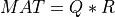
where Q is a pseudo-random orthogonal matrix following the Haar distribution from the group of orthogonal matrices and R is upper triangular.

The upper-diagonal elements of R follow the standard normal distribution and the squares of the diagonal elements of R, R(i,i)², follow a chi-squared distribution with n-i+1 degrees of freedom.

This subroutine uses a fast method based on Householder transformations for generating the first k columns of a n-by-n pseudo-random orthogonal matrices Q distributed according to the Haar measure over the orthogonal group of order n, in a factored form [Stewart:1980].

Synopsis:

call random_qr_cmp( mat(:n,:k) , diagr(:k) , beta(:k) , fillr=fillr , initseed=initseed )

ortho_gen_random_qr()

Purpose:

This subroutine generates the first k columns of a n-by-n real pseudo-random orthogonal matrix following the Haar distribution, which is defined as the product of n elementary Householder reflectors of order n and of a n-by-n diagonal matrix with diagonal elements equal to sign( one, DIAGR) [Stewart:1980]:

as returned by subroutine random_qr_cmp().

Synopsis:

call ortho_gen_random_qr( mat(:n,:k) , diagr(:k) , beta(:k) )

gen_random_sym_mat()

Purpose:

This subroutine generates a pseudo-random n-by-n real symmetric matrix with prescribed eigenvalues.

Optionally, the corresponding eigenvectors of the generated pseudo-random n-by-n real symmetric matrix can be computed if required.

Synopsis:

call gen_random_sym_mat( eigval(:k) , mat(:n,:n) , eigvec=eigvec(:n,:k) , initseed=initseed , hous=hous )

Examples:

ex1_gen_random_sym_mat.F90

ex1_trid_inviter.F90

ex1_trid_inviter_bis.F90

ex1_random_eig.F90

ex1_random_eig_pos.F90

ex1_random_eig_with_blas.F90

ex1_random_eig_pos_with_blas.F90

gen_random_mat()

Purpose:

This subroutine generates a pseudo-random m-by-n real matrix with prescribed singular values.

Optionally, the corresponding singular vectors of the generated pseudo-random m-by-n real matrix can be computed if required.

Synopsis:

call gen_random_mat( eigval(:k) , mat(:m,:n) , leftvec=leftvec(:m,:k) , rightvec=rightvec(:n,:k) , initseed=initseed , hous=hous )

Examples:

ex1_gen_random_mat.F90

ex1_rsvd_cmp.F90

ex1_rqr_svd_cmp.F90

ex1_rqlp_svd_cmp.F90

ex1_rqlp_svd_cmp2.F90

ex1_random_svd.F90

ex1_random_svd_with_blas.F90

ex1_random_svd_fixed_precision_with_blas.F90

gen_random_ortho_mat()

Purpose:

This function generates a pseudo-random m-by-n real matrix with with orthonormal columns. This pseudo-random m-by-n real matrix with orthonormal columns is generated as the first n columns of a m-by-m Householder matrix H.

Synopsis:

mat(:m,:n) = gen_random_ortho_mat( m , n , initseed=initseed )

Examples:

ex1_gen_random_ortho_mat.F90

partial_rqr_cmp()

Purpose:

partial_rqr_cmp() computes a (partial or full) QRCP or COD factorization of a real m-by-n matrix MAT using randomized techniques based on random Gaussian matrix projections [Duersch_Gu:2017] [Martinsson_etal:2017] [Xiao_etal:2017] [Duersch_Gu:2020]. MAT may be rank-deficient.

partial_rqr_cmp() performs the same task as qr_cmp2() and partial_qr_cmp() in module QR_Procedures, but are much faster, and also slightly less accurate, because of the use of randomization for selecting the pivot columns in the QRCP. The use of randomization for pivot selection in the QRCP algorithm allows to perform most of the parts of the algorithm mainly with matrix-matrix operations (e.g., “BLAS3”) as in the simple QR factorization without column pivoting (see the qr_cmp() subroutine in module QR_Procedures for more details).

The routine first computes a QRCP of MAT:

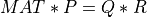
here P is n-by-n permutation matrix, which is computed by randomized techniques [Duersch_Gu:2017] [Xiao_etal:2017], R is an upper triangular or trapezoidal (if n>m) matrix and Q is a m-by-m orthogonal matrix.

At the user option, the QR factorization can be only partial, e.g., the subroutine ends when the numbers of selected columns of MAT is equal to a predefined value equals to kpartial = size(DIAGR) = size(BETA).

This leads implicitly to the following partition of Q:

where Q1 is a m-by-kpartial orthonormal matrix and Q2 is a m-by-(m-kpartial) orthonormal matrix orthogonal to Q1, and to the following corresponding partition of R:

where R11 is a kpartial-by-kpartial triangular matrix, R21 is zero by construction, R12 is a full kpartial-by-(n-kpartial) matrix and R22 is a full (m-kpartial)-by-(n-kpartial) matrix.

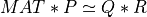
From these partitions of Q and R, we can obtain a good approximation of MAT of rank kpartial, since:

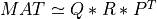
and, finally:

which is equivalent to assume that R22 is negligible.

If TAU is present, R12 is then annihilated by orthogonal transformations from the right, arriving at the partial COD:

where P is a n-by-n permutation matrix, Q1 is a m-by-kpartial orthonormal matrix, Z is a n-by-n orthogonal matrix and T11 is a kpartial-by-kpartial upper triangular matrix.

As in subroutine partial_qr_cmp(), if the optional argument TOL is present, calculations to determine the 1-norm condition number of R11 are performed and this condition number is used to determine the effective pseudo-rank of R11, krank. If this effective pseudo-rank is less than kpartial, which implies that the rank of MAT is also less than kpartial, the subroutine outputs a partial QR factorization corresponding to this effective pseudo-rank krank, instead of rank kpartial.

In all cases, the subroutine outputs krank (or kpartial if TOL is absent) in the argument KRANK and gives the error of the associated matrix approximation in the Frobenius norm, on exit.

Finally, note that partial_rqr_cmp() is an effective and efficient way for computing a low-rank approximation of MAT, but is less effective than partial_qr_cmp() to find the rank of MAT because of the use of randomization. As an illustration, the diagonal elements of R11 are not necessarily of decreasing absolute magnitude when computed by partial_rqr_cmp(), while this property is enforced with partial_qr_cmp(). See [Martinsson_etal:2017] [Xiao_etal:2017] for details. On the other hand, partial_qr_cmp() can be used safely for both tasks, but is much slower than partial_rqr_cmp().

Synopsis:

call partial_rqr_cmp( mat(:m,:n) , diagr(:kpartial) , beta(:kpartial) , ip(:n) , krank , tol=tol , tau=tau(:kpartial) , rng_alg=rng_alg , blk_size=blk_size , nover=nover )

Examples:

ex1_partial_rqr_cmp.F90

ex2_partial_rqr_cmp.F90

ex3_partial_rqr_cmp.F90

partial_rqr_cmp2()

Purpose:

partial_rqr_cmp2() computes a (partial or full) QRCP or COD factorization of a real m-by-n matrix MAT using randomized techniques based on random Gaussian matrix projections [Duersch_Gu:2017] [Martinsson_etal:2017] [Xiao_etal:2017] [Duersch_Gu:2020]. MAT may be rank-deficient.

In other words, partial_rqr_cmp2() performs the same task as partial_rqr_cmp() above. The main difference between the two subroutines is in the randomized technique for the pivot selection and the computation of the permutation matrix P. partial_rqr_cmp() uses an efficient updating formulae to recompute the compression matrix at each iteration (see [Duersch_Gu:2017] and [Xiao_etal:2017] for details) while partial_rqr_cmp2() regenerates the Gaussian and compression matrices at each iteration of the randomized (partial or full) blocked QRCP algorithm. This implies that partial_rqr_cmp() is usually faster than partial_rqr_cmp2() for very large matrices, but may be slightly less accurate in some cases.

The routine first computes a QRCP of MAT:

here P is n-by-n permutation matrix, which is computed by randomized techniques [Duersch_Gu:2017] [Xiao_etal:2017], R is an upper triangular or trapezoidal (if n>m) matrix and Q is a m-by-m orthogonal matrix.

At the user option, the QRCP factorization can be only partial, e.g., the subroutine ends when the numbers of selected columns of MAT is equal to a predefined value equals to kpartial = size(DIAGR) = size(BETA).

This leads implicitly to the following partition of Q:

where Q1 is a m-by-kpartial orthonormal matrix and Q2 is a m-by-(m-kpartial) orthonormal matrix orthogonal to Q1, and to the following corresponding partition of R:

where R11 is a kpartial-by-kpartial triangular matrix, R21 is zero by construction, R12 is a full kpartial-by-(n-kpartial) matrix and R22 is a full (m-kpartial)-by-(n-kpartial) matrix.

From these partitions of Q and R, we can obtain a good approximation of MAT of rank kpartial, since:

and, finally:

which is equivalent to assume that R22 is negligible.

If TAU is present, R12 is then annihilated by orthogonal transformations from the right, arriving at the partial COD factorization:

where P is a n-by-n permutation matrix, Q1 is a m-by-kpartial orthonormal matrix, Z is a n-by-n orthogonal matrix and T11 is a kpartial-by-kpartial upper triangular matrix.

As in subroutine partial_qr_cmp(), if the optional argument TOL is present, calculations to determine the 1-norm condition number of R11 are performed and this condition number is used to determine the effective pseudo-rank of R11, krank. If this effective pseudo-rank is less than kpartial, which implies that the rank of MAT is also less than kpartial, the subroutine outputs a partial QR factorization corresponding to this effective pseudo-rank krank, instead of rank kpartial.

In all cases, the subroutine outputs krank (or kpartial if TOL is absent) in the argument KRANK and gives the error of the associated matrix approximation in the Frobenius norm, on exit.

Finally, note that partial_rqr_cmp2() is an effective and efficient way for computing a low-rank approximation of MAT, but is less effective than partial_qr_cmp() to find the rank of MAT because of the use of randomization. As an illustration, the diagonal elements of R11 are not necessarily of decreasing absolute magnitude when computed by partial_rqr_cmp2(), while this property is enforced with partial_qr_cmp(). See [Martinsson_etal:2017] [Xiao_etal:2017] for details. On the other hand, partial_qr_cmp() can be used safely for both tasks, but is much slower than partial_rqr_cmp2().

Synopsis:

call partial_rqr_cmp2( mat(:m,:n) , diagr(:kpartial) , beta(:kpartial) , ip(:n) , krank , tol=tol , tau=tau(:kpartial) , rng_alg=rng_alg , blk_size=blk_size , nover=nover )

Examples:

ex1_partial_rqr_cmp2.F90

ex2_partial_rqr_cmp2.F90

ex3_partial_rqr_cmp2.F90

partial_rtqr_cmp()

Purpose:

partial_rtqr_cmp() computes an approximate partial and truncated QRCP factorization (or COD factorization) of a real m-by-n matrix MAT using randomization techniques:

here P is n-by-n permutation matrix, which is computed by randomized techniques [Mary_etal:2015], R is an upper triangular or trapezoidal kpartial-by-n matrix and Q is a m-by-kpartial matrix with orthonormal columns.

The randomized QRCP factorization is only partial and truncated, e.g., the subroutine ends when the numbers of columns of Q is equal to a predefined value equals to kpartial = size(DIAGR) = size(BETA). This leads implicitly to the following partition of R:

where R11 is a kpartial-by-kpartial triangular matrix and R12 is a full kpartial-by-(n-kpartial) matrix.

From this approximate partial and truncated QRCP factorization of MAT, partial_rtqr_cmp() can also estimate a partial and truncated orthogonal factorization of MAT. Thus, partial_rtqr_cmp() performs exactly the same tasks as partial_rqr_cmp() and partial_rqr_cmp2() subroutines and the arguments of partial_rtqr_cmp() are nearly the same as those in these two subroutines. However, partial_rtqr_cmp() is significantly faster when kpartial is relatively small and MAT is a very large matrix.

This is due to the fact that partial_rtqr_cmp() computes Q (in factored form), R11 and R12, but not R22 (where R22 is the bottom left (m-kpartial)-by-(n-kpartial) submatrix in the QR factorization of MAT) as partial_rqr_cmp() and partial_rqr_cmp2() subroutines. Furthermore, only an estimate of R12 is computed by partial_rtqr_cmp(), using a randomized algorithm described in [Mary_etal:2015], while the computation of R12 is exact in partial_rqr_cmp() and partial_rqr_cmp2() subroutines. Note also that partial_rtqr_cmp() does not recompute or update the compression matrix at each iteration as partial_rqr_cmp() and partial_rqr_cmp2(). See [Mary_etal:2015] [Duersch_Gu:2017] [Martinsson_etal:2017] [Xiao_etal:2017] [Duersch_Gu:2020] for more information.

All these features explain why partial_rtqr_cmp() is usually much faster than partial_rqr_cmp() and partial_rqr_cmp2() subroutines, but is also less accurate, especially for matrices with a slow decay of their singular values. See [Mary_etal:2015] for details.

Synopsis:

call partial_rtqr_cmp( mat(:m,:n) , diagr(:kpartial) , beta(:kpartial) , ip(:n) , krank , tol=tol , tau=tau(:kpartial) , rng_alg=rng_alg , niter=niter , nover=nover )

Examples:

ex1_partial_rtqr_cmp.F90

partial_rqr_cmp_fixed_precision()

Purpose:

partial_rqr_cmp_fixed_precision() computes a partial QRCP or COD factorization of a real m-by-n matrix MAT using randomized techniques:

here P is a n-by-n permutation matrix computed using randomization techniques, R is a kank-by-n upper triangular or trapezoidal matrix and Q is a m-by-krank with orthonormal columns. This leads to the following matrix approximation of MAT of rank krank:

krank is the target rank of the matrix approximation, which is sought, and this partial factorization must have an approximation error which fulfills:

where is the Frobenius norm and relerr is a prescribed accuracy tolerance for the relative error of the computed matrix approximation, specified in the input argument RELERR.

Thus, partial_rqr_cmp_fixed_precision() performs the same task as partial_rqr_cmp() and partial_rqr_cmp2(), but allows to stop the factorization at any stage in order to obtain a partial QRCP (or COD) factorization of MAT, which fullfills the above inequality.

In other words, krank, the rank of the matrix approximation, is not known in advance and is computed by the subroutine, while krank is fixed a priori and is an input argument in partial_rqr_cmp() and partial_rqr_cmp2() subroutines. Otherwise, all other arguments of partial_rqr_cmp_fixed_precision() have the same meaning as in partial_rqr_cmp() and partial_rqr_cmp2().

In all cases, on exit of partial_rqr_cmp_fixed_precision(), gives the error of the associated matrix approximation in the Frobenius norm and the associated relative error in the Frobenius norm is output in argument RELERR.

Note finally that partial_rqr_cmp_fixed_precision() performs exactly the same task as partial_qr_cmp_fixed_precision() subroutine in module QR_Procedures, but is much faster on large matrices because of the use of a randomized and blocked “BLAS3” algorithm instead of a standard “BLAS2” algorithm in partial_qr_cmp_fixed_precision(). Another difference is that, in partial_rqr_cmp_fixed_precision(), the rank of the matrix approximation is increased progressively of BLK_SIZE by BLK_SIZE until the prescribed tolerance for the relative error is satisfied while, in partial_qr_cmp_fixed_precision(), the rank of the matrix approximation is increased one by one until the prescribed tolerance for the relative error is satisfied. In other words, the rank of the matrix approximation found by partial_rqr_cmp_fixed_precision() is always larger than the one found by partial_qr_cmp_fixed_precision() and is a multiple of BLK_SIZE.

Synopsis:

call partial_rqr_cmp_fixed_precision( mat(:m,:n) , relerr , diagr(:min(m,n)) , beta(:min(m,n)) , ip(:n) , krank , tau=tau(:min(m,n)) , rng_alg=rng_alg , blk_size=blk_size , nover=nover )

Examples:

ex1_partial_rqr_cmp_fixed_precision.F90

rqb_cmp()

Purpose:

rqb_cmp() computes a (partial or full) QB factorization of a real m-by-n matrix MAT using randomized power or subspace iteration techniques [Halko_etal:2011] [Gu:2015] [Martinsson:2019]:

Here, Q is a m-by-nqb orthonormal matrix, B is a nqb-by-n and the product is a good approximation of MAT according to the spectral or Frobenius norm. nqb is the target rank of the partial QB decomposition, which is sought, and is equal to the number of columns of the output real matrix argument Q, i.e., nqb = size( Q, 2 ).

At the user option, an approximate QR (eventually with column pivoting) or COD factorization of MAT can be derived from this initial QB factorization with the help of optional arguments in rqb_cmp() subroutine.

Synopsis:

call rqb_cmp( mat(:m,:n) , q(:m,:nqb) , b(:nqb,:n) , niter=niter , rng_alg=rng_alg , ortho=ortho , comp_qr=com_qr , ip=ip(:n) , tol=tol , tau=tau(:nqb) )

Examples:

ex1_rqb_cmp.F90

ex1_rqb_solve.F90

rqb_cmp_fixed_precision()

Purpose:

rqb_cmp_fixed_precision() computes a partial QB factorization of a real m-by-n matrix MAT using randomized power or subspace iteration techniques [Halko_etal:2011] [Gu:2015] [Martinsson_Voronin:2016] [Yu_etal:2018] [Martinsson:2019]:

Here, Q is a m-by-nqb orthonormal matrix, B is a nqb-by-n and the product is a good approximation of MAT according to the spectral or Frobenius norm. nqb is the target rank of the partial QB decomposition, which is sought, and this partial factorization must have an approximation error which fulfills:

where is the Frobenius norm and relerr is a prescribed accuracy tolerance for the relative error of the computed partial QB approximation in the Frobenius norm, specified as an argument (e.g., argument RELERR) in the call to rqb_cmp_fixed_precision().

In other words, nqb is not known in advance and is determined in the subroutine. This explains why the output real array arguments Q and B, which contain the computed partial QB factorization, must be declared in the calling program as pointers.

rqb_cmp_fixed_precision() searches incrementally the best (e.g., smallest) partial QB approximation, which fulfills the prescribed accuracy tolerance for the relative error based on an improved version of the randQB_FP algorithm described in [Yu_etal:2018]. See also [Martinsson_Voronin:2016]. More precisely, the rank of the partial QB approximation is increased progressively of BLK_SIZE by BLK_SIZE until the prescribed accuracy tolerance is satisfied and then improved and adjusted precisely by additional subspace iterations (as specified by the optional NITER_QB integer argument) to obtain the smallest partial QB approximation, which satisfies the prescribed tolerance.

Note that the product of the two integer arguments BLK_SIZE and MAXITER_QB (see below for their precise meaning), determines the maximum allowable rank of the matrix approximation, which is sought.

On exit, nqb = size( Q, 2 ), e.g., nqb is equal to the number of columns of the output real matrix pointer argument Q, which contains the computed orthonormal matrix Q and the relative error in the Frobenius norm of the computed partial QB approximation is output in argument RELERR.

At the user option, an approximate QR (eventually with column pivoting) or COD factorization of MAT can be derived from this initial QB factorization with the help of optional arguments in rqb_cmp_fixed_precision() subroutine.

Note, finally, that if you already know the rank of the partial QB approximation of MAT you are seeking, it is better to use rqb_cmp() rather than rqb_cmp_fixed_precision() as rqb_cmp() is faster and slightly more accurate.

Synopsis:

call rqb_cmp_fixed_precision( mat(:m,:n) , relerr , q(:,:) , b(:,:) , failure_relerr=failure_relerr , niter=niter , rng_alg=rng_alg , blk_size=blk_size , maxiter_qb=maxiter_qb , ortho=ortho , reortho=reortho , niter_qb=niter_qb , comp_qr=com_qr , ip=ip(:n) , tol=tol , tau=tau(:nqb) )

Examples:

ex1_rqb_cmp_fixed_precision.F90

id_cmp()

Purpose:

id_cmp() computes a (partial) column Interpolative Decomposition (ID) of a m-by-n real matrix MAT. A column ID factorization of rank krank approximates MAT as:

where C is an m-by-krank matrix, which consists of a subset of krank columns of MAT and V is a krank-by-n matrix, which contains a krank-by-krank identity matrix as a submatrix. The subset of the columns of MAT, which forms C, is selected to give a good approximation of MAT in the spectral or Frobenius norm.

Such column ID factorization can be computed with the help of a (deterministic or randomized) partial QRCP factorization of MAT. See the detailed description of id_cmp() and [Stewart:1999] [Berry_etal:2005] [Voronin_Martinsson:2015] [Voronin_Martinsson:2017] [Martinsson:2019] for more information.

Synopsis:

call id_cmp( mat(:m,:n) , ip(:n) , t(:krank,:n-krank) , c=c(:krank,:n) , v=v(:krank,:n) , rnorm=rnorm , diagr=diagr(:krank) , beta=beta(:krank) , tol=tol , random_qr=random_qr , rng_alg=rng_alg , blk_size=blk_size , nover=nover )

Examples:

ex1_id_cmp.F90

ts_id_cmp()

Purpose:

ts_id_cmp() computes a (partial) two-sided Interpolative Decomposition (tsID) of a m-by-n real matrix MAT. A tsID factorization of rank krank approximates a real matrix MAT as a triple matrix product:

where W is an m-by-krank matrix, V is a krank-by-n matrix and MAT_skel is a squared krank-by-krank matrix, the so-called “skeleton” of MAT. W, V and MAT_skel are estimated to give a good approximation of MAT in the spectral or Frobenius norm.

Such tsID factorization can be computed with the help of a (deterministic or randomized) partial QRCP factorization of MAT and of a matrix derived from its partial QR decomposition, more precisely with a column ID of MAT and a row ID of a subset of the columns of MAT. See the detailed description of ts_id_cmp() and [Stewart:1999] [Berry_etal:2005] [Voronin_Martinsson:2015] [Voronin_Martinsson:2017] [Martinsson:2019] for more information.

Synopsis:

call ts_id_cmp( mat(:m,:n) , ip_row(:m) , ip_col(:n) , w(:m,:krank) , v=v(:krank,:n) , skelmat(:krank,:krank) , rnorm=rnorm , diagr=diagr(:krank) , beta=beta(:krank) , tol=tol , random_qr=random_qr , rng_alg=rng_alg , blk_size=blk_size , nover=nover )

Examples:

ex1_ts_id_cmp.F90

cur_cmp()

Purpose:

cur_cmp() computes a (partial) CUR Decomposition (tsID) of a m-by-n real matrix MAT. A CUR factorization of rank krank approximates a real matrix MAT as a triple matrix product:

where C and R are m-by-krank and krank-by-n matrices, which are, respectively, subsets of the columns and rows of MAT, and U is a krank-by-krank, which is estimated to make the matrix product a good approximation of MAT according to the Frobenius norm. The CUR factorization is an important tool for handling large-scale data sets, offering several advantages over the Singular Value Decomposition (SVD): the columns and rows that comprise C and R are representative of the data and they are sparse if MAT is sparse. See [Mahoney_Drineas:2009] and [Martinsson:2019] for a discussion.

Computing an approximate CUR decomposition is generally a three-step process. The C and R matrix factors in the CUR factorization can be first estimated with the help of (randomized or deterministic) partial QRCP factorizations of MAT and , respectively. In a final step, we then seek a krank-by-krank matrix U such that:

See the detailed description of cur_cmp() and [Stewart:1999] [Berry_etal:2005] [Voronin_Martinsson:2017] [Martinsson:2019] for more information on the algorithm used to estimate the matrices C, U and R of the CUR factorization.

Synopsis:

call cur_cmp( mat(:m,:n) , ip_row(:m) , ip_col(:n) , u(:krank,:krank) , c=c(:m,:krank) , r=r(:krank,:n) , rnorm_row=rnorm_row , rnorm_col=rnorm_col , tol=tol , random_qr=random_qr , rng_alg=rng_alg , blk_size=blk_size , nover=nover )

Examples:

ex1_cur_cmp.F90

simple_shuffle()

Purpose:

This generic subroutine shuffles all the elements of the vector VEC.

Synopsis:

call simple_shuffle( vec(:) ) ! vec is a real     vector of kind stnd
call simple_shuffle( vec(:) ) ! vec is a complex  vector of kind stnd
call simple_shuffle( vec(:) ) ! vec is an integer vector of kind i4b

drawsample()

Purpose:

This subroutine may be used to draw a sample, without replacement of size NSAMPLE from a population of size SIZE(POP). On output, the integer vector POP(1:NSAMPLE) indicates which observations are included in the sample.

The integer vector POP must be dimensioned at least as large as NSAMPLE in the calling program.

Synopsis:

call drawsample( nsample , pop(:) ) ! pop is an integer vector of kind i4b

Examples:

ex1_drawsample.F90

ex2_drawsample.F90

drawbootsample()

Purpose:

This subroutine may be used to draw a bootstrap random sample of size SIZE(SAMPLE) from a finite population of size NPOP. On output, the integer vector SAMPLE indicates which observations are included in the bootstrap sample.

The sampling is done with replacement, meaning that the sample may contain duplicate observations.

Synopsis:

call drawbootsample( npop , sample(:) ) ! sample is an integer vector of kind i4b