MODULE QR_Procedures
Module QR_Procedures exports subroutines for computing (full or partial) QR and LQ decompositions and related factorizations or computations.
A general rectangular m-by-n matrix MAT has a QR decomposition into the product of an orthogonal
m-by-m square matrix Q (where  ) and a
 m-by-n upper-triangular
(or upper trapezoidal) matrix R [Lawson_Hanson:1974] [Golub_VanLoan:1996] [Hansen_etal:2012],
Similarly, MAT has a LQ decomposition into the product of a m-by-n lower-triangular (or lower trapezoidal)
matrix L and an orthogonal n-by-n square matrix Q (where ) [Lawson_Hanson:1974]
[Golub_VanLoan:1996],
The QR decomposition can be used to convert a full rank n-by-n linear system  into the triangular
system
into the triangular
system  , which can be solved by back-substitution.
Similarly, the LQ decomposition can be used to convert a full rank n-by-n linear system 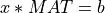 into the triangular
system
into the triangular
system 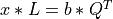 , which can also be solved by back-substitution.
The QR or LQ decompositions can also be used to solve linear least squares problems, when MAT has full
rank [Lawson_Hanson:1974] [Golub_VanLoan:1996] [Hansen_etal:2012].
See the module LLSQ_Procedures for more details.
Another use of the QR or LQ decompositions is to compute an orthonormal basis for a set of vectors. The first min(m,n) columns
of Q of the QR decomposition form an orthonormal basis for the range of MAT,  , when
 MAT has full
rank. Similarly, the first min(m,n) rows of Q of the LQ decomposition form an orthonormal basis for the range of
MATT, when MAT has full rank.
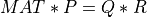
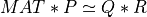
The QR decomposition of a m-by-n matrix MAT can be extended to the rank deficient case by introducing a column
permutation P [Lawson_Hanson:1974] [Golub_VanLoan:1996] [Hansen_etal:2012],
![MAT * P = Q * R = Q * \left[ \begin{matrix} R11 & R12 \\ 0 & R22 \end{matrix} \right] \simeq \left[ \begin{matrix} R11 & R12 \\ 0 & 0 \end{matrix} \right]](../_images/math/2e28e8398fb229fa1b8b694d005d0db916df4a46.png)
where P is a permutation of the columns of In, the identity matrix of order n, R11 is a r-by-r
full rank upper triangular matrix, R12 is a r-by-n-r matrix and R22 is a (m-r)-by-(n-r) upper
triangular matrix, which is almost negligible. In other words, when MAT is rank deficient with 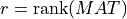 , the matrix
 R
can be partitioned into four submatrices and the dimension of R11 is equal to  . The effective rank of
 MAT, r,
can be estimated by the routines provided here.
When MAT is square and of full rank (e.g., r = m = n), this decomposition can also be used to convert the linear system
into the triangular system 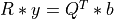 ,
,  , which can be solved by back-substitution and permutation.
More generally, for a matrix with column rank r, The first r columns of Q form an orthonormal basis for the range of MAT
and the QR decomposition with Column Pivoting (QRCP) can be used to solve rank deficient linear least squares problems. See the manual of the module
LLSQ_Procedures for more details.
Finally, the Complete Orthogonal Decomposition (COD) of a m-by-n matrix MAT [Lawson_Hanson:1974] [Golub_VanLoan:1996]
[Hansen_etal:2012] is a generalization of the QRCP described above, given by

where P is a n-by-n permutation matrix, Q is a m-by-m orthogonal matrix,
Z is a n-by-n orthogonal matrix and T is a m-by-n matrix.
If MAT has full column rank, then T = R, Z = I and this reduces to the QRCP.
On the other hand, if MAT is column deficient, T has the form:
![T =
\left[
\begin{matrix}
T11 & 0 \\
0 & 0
\end{matrix}
\right]](../_images/math/b28c5d6968ecfbe7d45c68b3300ddbc0a2d0a6be.png)
where T11 is a r-by-r upper triangular full rank matrix and r is the effective rank of MAT.
The advantage of using the COD for rank deficient matrices is the ability to compute the minimum norm solution
to the linear least squares problem 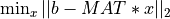 . See description of the routines in
module LLSQ_Procedures for more details.
. See description of the routines in
module LLSQ_Procedures for more details.
All these different matrix decompositions can be performed with routines available in this module. Moreover, most routines in this module are blocked and multi-threaded versions [Walker:1988] [Dongarra_etal:1989] of the standard sequential algorithms for the QR, LQ, QRCP and COD decompositions [Lawson_Hanson:1974] [Golub_VanLoan:1996]. All routines available in module QR_Procedures are deterministic, but randomized full or partial QRCP and COD decompositions [Duersch_Gu:2017] [Martinsson_etal:2017] [Duersch_Gu:2020] [Martinsson:2019], which perform the same tasks and are much faster than their deterministic versions, are also available in module Random and can be used efficiently for very large matrices.
Please note, finally, that routines provided in this module apply only to real data types.
In order to use one of these routines, you must include an appropriate use QR_Procedures or use Statpack statement
in your Fortran program, like:
use QR_Procedures, only: lq_cmp
or :
use Statpack, only: lq_cmp
Here is the list of the public routines exported by module QR_Procedures:
-
lq_cmp()
Purpose:
lq_cmp() computes a LQ factorization of a real m-by-n matrix MAT :
where Q is orthogonal and L is lower trapezoidal (lower triangular if m<=n).
Synopsis:
call lq_cmp( mat(:m,:n) , diagl(:min(m,n)) , tau(:min(m,n)) , use_qr=use_qr )
Examples:
-
ortho_gen_lq()
Purpose:
ortho_gen_lq() generates an m-by-n real matrix with orthonormal rows, which is
defined as the first m rows of a product of k elementary reflectors of order n

as returned by lq_cmp().
Synopsis:
call ortho_gen_lq( mat(:m,:n) , tau(:p) , use_qr=use_qr )
Examples:
-
apply_q_lq()
Purpose:
apply_q_lq() overwrites the general real m-by-n matrix C with
 if LEFT =
 trueand TRANS =false, if LEFT =
 trueand TRANS =true, if LEFT =
 falseand TRANS =false, if LEFT =
 falseand TRANS =true,
where Q is a real orthogonal matrix defined as the product of k
elementary reflectors

as returned by lq_cmp(). Q is of order m if LEFT = true and of order n
if LEFT = false.
Synopsis:
call apply_q_lq( mat(:m,:n) , tau(:p) , c(:n)      ,        trans )
call apply_q_lq( mat(:m,:n) , tau(:p) , c(:mc,:nc) , left , trans )
-
qr_cmp()
Purpose:
qr_cmp() computes a QR factorization of a real m-by-n matrix MAT :
where Q is orthogonal and R is upper trapezoidal (upper triangular if m>=n).
Synopsis:
call qr_cmp( mat(:m,:n) , diagr(:p) , beta(:p) )
Examples:
-
qr_cmp2()
Purpose:
qr_cmp2() computes a (complete) orthogonal factorization of a real m-by-n matrix
MAT. MAT may be rank-deficient. The routine first computes a QRCP of MAT:
here P is n-by-n permutation matrix, R is an upper triangular or trapezoidal
(if n>m) matrix and Q is a m-by-m orthogonal matrix.
R can then be partitioned by defining R11 as the largest leading squared submatrix of R whose
estimated condition number, in the 1-norm, is less than 1/TOL (or such that  if the argument TOL is absent). The order of
 R11, krank, is the effective rank of MAT.
This leads to the following partition of R:
![R = \left[ \begin{matrix} R11 & R12 \\ 0 & R22 \end{matrix} \right] \simeq \left[ \begin{matrix} R11 & R12 \\ 0 & 0 \end{matrix} \right]](../_images/math/4ff8969eef4efe909404b1c832ad2f50a1f07156.png)
where R22 can be considered to be negligible.
If TAU is present, R22 is considered to be negligible and R12 is annihilated
by orthogonal transformations from the right, arriving at the complete orthogonal factorization:
![MAT * P \simeq Q * \left[ \begin{matrix} T11 & 0 \\ 0 & 0 \end{matrix} \right] * Z](../_images/math/fd164e159953d8face4b81a106a7c56e5ad5c2de.png)
where P is a n-by-n permutation matrix, Q is a m-by-m orthogonal matrix,
Z is a n-by-n orthogonal matrix and T11 is a krank-by-krank upper
triangular matrix.
Note, finally, that randomized versions of subroutine qr_cmp2() are available in module Random, which perform
the same tasks with nearly the same accuracy and are much faster. qr_cmp2() uses a standard “BLAS2” algorithm without any blocking
and is thus not optimized for computing QRCP or COD factorizations of very large matrices.
For large matrices, subroutines partial_rqr_cmp() and partial_rqr_cmp2() in module Random, which
use randomized blocked “BLAS3” algorithms described in [Duersch_Gu:2017] [Martinsson_etal:2017] [Xiao_etal:2017] [Duersch_Gu:2020],
are a much better choice.
Synopsis:
call qr_cmp2( mat(:m,:n) , diagr(:min(m,n)) , beta(:min(m,n)) , ip(:n) , krank , tol=tol , tau=tau(:min(m,n)) )
Examples:
-
partial_qr_cmp()
Purpose:
partial_qr_cmp() computes a (partial) QRCP or COD of a real m-by-n matrix MAT. MAT may be rank-deficient.
In other words, partial_qr_cmp() performs the same task as qr_cmp2() above, but allows to stop the
factorization at any stage in order to obtain only a partial QRCP or COD factorization of MAT.
This option is not allowed with qr_cmp2(), which always computes a full QRCP in its first stage.
The routine first computes a QRCP of MAT:
here P is n-by-n permutation matrix, R is an upper triangular or trapezoidal
(if n>m) matrix and Q is a m-by-m orthogonal matrix.
At the user option, the QR factorization can be only partial, e.g., the subroutine ends when the numbers of selected columns
of MAT for pivot selection is equal to a predefined value equals to kpartial = size(DIAGR) = size(BETA).
This leads implicitly to the following partition of Q:
![Q = \left[ \begin{matrix} Q1 & Q2 \end{matrix} \right]](../_images/math/8a287b679be074d9a0230a7fc886542233fc5127.png)
where Q1 is a m-by-kpartial orthonormal matrix and Q2 is a m-by-(m-kpartial)
orthonormal matrix orthogonal to Q1, and to the following corresponding partition of R:
![R = \left[ \begin{matrix} R11 & R12 \\ 0 & R22 \end{matrix} \right]](../_images/math/eeaae8fde5702c4eac26439ddd46e8e67f6b0886.png)
where R11 is a kpartial-by-kpartial triangular matrix, R21 is zero by construction,
R12 is a full kpartial-by-(n-kpartial) matrix and R22 is a full (m-kpartial)-by-(n-kpartial)
matrix.
From these partitions of Q and R, we can obtain a good approximation of MAT of rank kpartial, since:
![MAT * P \simeq Q1 * \left[ \begin{matrix} R11 & R12 \end{matrix} \right]](../_images/math/627e18dd959e219954596a4e04fb91a3c43c3ab6.png)
and, finally:
![MAT \simeq Q1 * \left[ \begin{matrix} R11 & R12 \end{matrix} \right]* P^T](../_images/math/36403307da8197c5804892cf5f872c4b5d801f32.png)
which is equivalent to assume that R22 is negligible.
If TAU is present, R12 is then annihilated by orthogonal transformations from the right, arriving at the partial orthogonal factorization:
![MAT * P \simeq Q1 * \left[ \begin{matrix} T11 & 0 \end{matrix} \right] * Z](../_images/math/658023e7066324e101f6b1d75429f88d52b15533.png)
where P is a n-by-n permutation matrix, Q1 is a m-by-kpartial orthonormal matrix,
Z is a n-by-n orthogonal matrix and T11 is a kpartial-by-kpartial upper
triangular matrix.
As in subroutine qr_cmp2(), if the optional argument TOL is present, calculations to determine the 1-norm condition number of R11
are performed and this condition number is used to determine the effective pseudo-rank of R11, krank. If this effective pseudo-rank
is less than kpartial, which implies that the rank of MAT is also less than kpartial, the subroutine outputs a partial QR factorization
corresponding to this effective pseudo-rank krank, instead of rank kpartial.
In all cases, the subroutine outputs krank (or kpartial if TOL is absent) in the argument KRANK and
 gives the error of the associated matrix approximation in the Frobenius norm, on exit.
Note, finally, that randomized versions of subroutine partial_qr_cmp() are available in module Random, which perform
the same tasks with nearly the same accuracy and are much faster. partial_qr_cmp() uses a standard “BLAS2” algorithm without any blocking
and is thus not optimized for computing a partial QRCP or COD of very large matrices.
For large matrices, subroutines partial_rqr_cmp() and partial_rqr_cmp2() in module Random, which
use randomized blocked “BLAS3” algorithms described in [Duersch_Gu:2017] [Martinsson_etal:2017] [Xiao_etal:2017] [Duersch_Gu:2020],
are a much better choice.
Synopsis:
call partial_qr_cmp( mat(:m,:n) , diagr(:kpartial) , beta(:kpartial) , ip(:n) , krank , tol=tol , tau=tau(:kpartial) )
Examples:
-
partial_qr_cmp_fixed_precision()
Purpose:
partial_qr_cmp_fixed_precision() computes a partial QRCP (or COD) of a real m-by-n matrix MAT:
here P is a n-by-n permutation matrix, R is a kank-by-n upper triangular or trapezoidal
matrix and Q is a m-by-krank with orthonormal columns. This leads to the following matrix approximation
of MAT of rank krank:
krank is the target rank of the matrix approximation, which is sought, and this partial factorization must have an
approximation error which fulfills:

where  is the Frobenius norm and
 relerr is a prescribed accuracy tolerance for the relative error of the computed
matrix approximation, specified in the input argument RELERR.
Thus, partial_qr_cmp_fixed_precision() performs exactly the same task as partial_qr_cmp() above, but allows to stop the
factorization at any stage in order to obtain a partial QR (or orthogonal) factorization of MAT, which fullfills the
above inequality.
In other words, krank, the rank of the matrix approximation, is not known in advance and is computed by the subroutine.
Otherwise, all other arguments of partial_qr_cmp_fixed_precision() have the same meaning as in qr_cmp2() or partial_qr_cmp().
In all cases, on exit, gives the error of the associated matrix approximation in the Frobenius norm and
the associated relative error in the Frobenius norm is output in argument RELERR.
Note, finally, that a randomized version of subroutine partial_qr_cmp_fixed_precision() is available in module Random,
which performs the same tasks with nearly the same accuracy and is much faster. partial_qr_cmp_fixed_precision() uses a standard “BLAS2” algorithm
without any blocking and is thus not optimized for computing partial QRCPs or CODs of very large matrices.
For large matrices, subroutine partial_rqr_cmp_fixed_precision() in module Random, which uses a randomized blocked “BLAS3”
algorithm described in [Duersch_Gu:2017] [Martinsson_etal:2017] [Xiao_etal:2017] [Duersch_Gu:2020], is a much better choice.
Synopsis:
call partial_qr_cmp_fixed_precision( mat(:m,:n) , relerr , diagr(:min(m,n)) , beta(:min(m,n)) , ip(:n) , krank , tau=tau(:min(m,n)) )
Examples:
ex1_partial_qr_cmp_fixed_precision.F90
-
qrfac()
Purpose:
qrfac() is a low level subroutine for computing a (complete) orthogonal factorization
of the array section SYST(1:m,1:n) where n <= size(SYST,2) and
m = size(SYST,1).
The routine first computes a QRCP:

where P is n-by-n permutation matrix, R is an upper triangular or trapezoidal
(if n>m) matrix and Q is a m-by-m orthogonal matrix.
The orthogonal transformation Q is then applied to SYST(1:m,n+1:):

Then, the rank of SYST(1:m,1:n) is determined by finding the squared submatrix R11 of R
which is defined as the largest leading submatrix whose estimated condition
number, in the 1-norm, is less than 1/TOL or such that if TOL
is absent. The order of R11, krank, is the effective rank of SYST(1:m,1:n).
This leads to the following partition of R:
where R22 can be considered to be negligible.
If MIN_NORM = true, R22 is considered to be negligible and R12 is annihilated by orthogonal
transformations from the right, arriving at the complete orthogonal factorization:
![SYST(1:m,1:n) * P \simeq Q * \left[ \begin{matrix} T11 & 0 \\ 0 & 0 \end{matrix} \right] * Z](../_images/math/54c1213187a03769757fb1835105657433561709.png)
where P is a n-by-n permutation matrix, Q is a m-by-m orthogonal matrix,
Z is a n-by-n orthogonal matrix and T11 is a krank-by-krank upper
triangular matrix.
Synopsis:
call qrfac( name_proc , syst(:m,:n) , kfix , krank , min_norm, diagr(:) , beta(:) , h(:) , tol=tol , ip=ip(:) )
-
ortho_gen_qr()
Purpose:
ortho_gen_qr() generates an m-by-n real matrix with orthonormal columns, which is
defined as the first n columns of a product of k elementary reflectors of order m

as returned by qr_cmp() or qr_cmp2().
Synopsis:
call ortho_gen_qr( mat(:m,:n) , beta(:p) )
Examples:
-
apply_q_qr()
Purpose:
apply_q_qr() overwrites the general real m-by-n matrix C with
- if LEFT =
trueand TRANS =false, - if LEFT =
trueand TRANS =true, - if LEFT =
falseand TRANS =false, - if LEFT =
falseand TRANS =true,
where Q is a real orthogonal matrix defined as the product of k
elementary reflectors
as returned by qr_cmp() or qr_cmp2(). Q is of order m if LEFT = true
and of order n if LEFT = false.
Synopsis:
call apply_q_qr( mat(:m,:n) , beta(:p) , c(:m)      ,        trans )
call apply_q_qr( mat(:m,:n) , beta(:p) , c(:mc,:nc) , left , trans )
Examples: