MODULE FFT_Procedures
Module FFT_Procedures exports routines for (Fast) Fourier Transform (FFT) computations.
A large part of the documentation of this module is adapted from the nice documentation of the GNU Scientific Library [gsl].
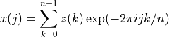
Before going to the FFT, let us first briefly recall the Discrete Fourier Transform (DFT) [Bloomfield:1976] [Oppenheim_Schafer:1999]. For a complex valued sequence z(k) with length n, its n-point DFT is defined as,
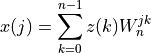
for 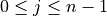 and where
 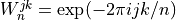 with
with  and
and
 . The key properties of the DFT are based on the following elementary identity
for and where  takes
takes  when
when  =
=  and otherwise.
The naive evaluation of the discrete Fourier transform is thus a matrix-vector multiplication
and otherwise.
The naive evaluation of the discrete Fourier transform is thus a matrix-vector multiplication  , which takes
 operations for a
 n-valued complex sequence [Bloomfield:1976] [Oppenheim_Schafer:1999].
FFTs are efficient algorithms for computing the DFT, which use cleaver divide-and-conquer strategies to factorize the
matrix  into smaller sub-matrices, corresponding to the integer factors of the length
  .
If can be factorized into a product of integers
.
If can be factorized into a product of integers  then the DFT can be
computed in
then the DFT can be
computed in  operations. For a radix-
2 FFT, this gives an operation count of
 [Bloomfield:1976] [Oppenheim_Schafer:1999].
The module FFT_Procedures exports general routines, which work for complex valued arrays of any length. FFT routines for real valued sequences are also provided, but for real arrays of even length only (or of any length, but for a pair of real valued sequences of the same size). Routines for the FFT of complex and real arrays of up to three dimensions are also included.
Finally, DFTs for real sequences of any length, based on the Goertzel method, are also available here [Goertzel:1958] [Oppenheim_Schafer:1999]. This method is competitive with the FFT for the DFT of short sequences only.
Depending on the shape of the complex valued array to be transformed, a radix-2 decimation-in-time Cooley-Tukey
algorithm [Cooley_etal:1969] [Oppenheim_Schafer:1999], Bailey’s Four-Step FFT algorithm [Bailey:1990] or a CHIRP-Z
transform [Monro_Branch:1977] are used/combined to compute the complex or real FFTs. The radix-2 decimation-in-time
algorithm works only for lengths which are a power of two, but combined with the two other methods, this gives FFTs for complex
arrays of any length.
At the user level, the routines provided here offer two types of transforms for complex and real sequences: forwards and backwards.
Our definition of the forward Fourier transform,  , is,
, is,
for and our definition of the backward-inverse Fourier transform,
 , is,
, is,
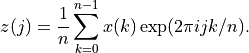
for . The factor of  makes this transform a true inverse. For example, a call
to
makes this transform a true inverse. For example, a call
to fft() with FORWARD = true followed by a call to
fft() with FORWARD = false should return the original complex data (within
numerical errors).
The following fragment of code illustrates how easy it it to compute the FFT of a complex valued sequence with the STATPACK FFT routines:
use FFT_Procedures, only: init_fft, fft
...
integer(i4b), parameter :: n=300
...
real(stnd), dimension(n) :: vec, vect
...
!
call init_fft( n )                                ! Initialize the fft computations
call real_fft( vec(:n), vect(:n), forward=true )  ! Perform a forward fft, output argument vect(:n) contains the forward FFT of vec(:n)
!
call end_fft( )                                   ! Deallocate internal fft workspace
For physical applications, it is important to remember that the index
appearing in the DFT does not correspond directly to a physical
frequency. If the time-step of the DFT is  then the
frequency-domain includes both positive and negative frequencies,
ranging from
then the
frequency-domain includes both positive and negative frequencies,
ranging from  through 0 to
  .
.
In the STATPACK FFT routines the positive frequencies are stored from the beginning of the output array argument up to the middle, and the negative frequencies are stored backwards from the end of the array.
Here is a table, which shows the correspondence between the time-domain data  and the
frequency-domain data
and the
frequency-domain data  , used in the STATPACK FFT routines (note that the index runs
from to
, used in the STATPACK FFT routines (note that the index runs
from to  as in our definition of the DFT):
index    z               x = FFT(z)

0        z(t = 0)        x(f = 0)
1        z(t = 1)        x(f = 1/(n Delta))
2        z(t = 2)        x(f = 2/(n Delta))
.        ........        ..................
n/2      z(t = n/2)      x(f = +1/(2 Delta),
                               -1/(2 Delta))
.        ........        ..................
n-3      z(t = n-3)      x(f = -3/(n Delta))
n-2      z(t = n-2)      x(f = -2/(n Delta))
n-1      z(t = n-1)      x(f = -1/(n Delta))
When is even the location  contains the most positive
and negative frequencies (
contains the most positive
and negative frequencies ( ,
,  )
which are equivalent. If is odd then general structure of the
table above still applies, but does not appear.
Remind, finally, that the indexing in the above table is shifted by one compared to
the classical Fortran convention.
)
which are equivalent. If is odd then general structure of the
table above still applies, but does not appear.
Remind, finally, that the indexing in the above table is shifted by one compared to
the classical Fortran convention.
The routines for real valued sequences are similar to those for complex sequences. However, there is an important difference because the Fourier transform of a real sequence is a complex sequence with a special symmetry:
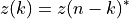
A sequence with this symmetry is called conjugate-complex or half-complex. This symmetry of the half-complex sequence
implies that only half of the complex numbers need to be computed and stored. The remaining half can
be reconstructed using the half-complex symmetry property. This explains, for example, why the output complex argument VECT of
the routine real_fft(), which computes the FFT of a n-element real sequence vec, has a size of size(vec)/2 + 1
for a real valued sequence of even length size(vec).
The STATPACK FFT routines for a real valued sequence of even length, compute and store only the coefficients of the positive
frequency half of the full complex Fourier transform of the input real valued sequence (see the table above). From this output
half-complex sequence, the full complex Fourier transform of the input real valued sequence vec of even length n
can be easily computed as illustrated by the following portion of code:
use FFT_Procedures, only: init_fft, real_fft
...
integer(i4b), parameter :: n=300, nd2 = n/2   ! n is even
...
real(stnd),    dimension(200) :: vec
complex(stnd), dimension(200) :: vect
...
!
call init_fft( nd2 )                                  ! Initialize the real fft computations
call real_fft( vec(:n), vect(:nd2+1), forward=true )  ! Performs the real fft, argument vect(:nd2+1) is the output half-complex sequence
!
vect(n:nd2+2:-1) = conjg( vect(2:nd2) )               ! Compute the full complex Fourier transform of vec(:n) using the symmetry
!
call end_fft( )                                       ! Deallocate internal fft workspace
Note also that routines, which compute directly the backward-inverse Fourier transform (which is a real sequence) of an half-complex sequence,
are not provided in this version STATPACK. The generic real_fft() routine does provide a backward Fourier transform for a real valued sequence,  ,
based on the following formula:
,
based on the following formula:
But, the result is again a half-complex sequence and this is not the real backward-inverse Fourier transform of the half-complex sequence obtained by a call
to real_fft() with FORWARD = true.
Please note that routines provided in this module apply only to real/complex data of kind stnd. The real/complex kind type stnd is defined in module Select_Parameters.
In order to use one of these routines, you must include an appropriate use FFT_Procedures or use Statpack statement
in your Fortran program, like:
use FFT_Procedures, only: init_fft
or:
use Statpack, only: init_fft
Here is the list of the public routines exported by module FFT_Procedures:
-
init_fft()
Purpose:
init_fft() sets up constants, the Chirp functions and the Fourier transform of the Chirp functions for use by other STATPACK FFT routines, which compute the FFT for a complex (or real) valued array.
init_fft() is first called to establish and transform the Chirp functions and other constants. Then, STATPACK FFT routines can be called any number of times without the precalculated constants being destroyed; a further call to init_fft() will only be necessary if Fourier transforms for a new length (or shape) are required.
Synopsis:
call init_fft ( shap(:n), dim=dim )
call init_fft ( length1 )
call init_fft ( length1, length2 )
call init_fft ( length1, length2, length3 )
Examples:
-
fftxy()
Purpose:
Given two real valued sequences (arrays) of the same length (shape), X and Y, fftxy() returns the Fast Fourier Transforms (FFT) of these sequences (arrays) in the two complex valued sequences (arrays) FFTX and FFTY.
Real arrays of up to three dimensions can be FFT by fftxy(). For arrays of two or three dimensions, the FFTs can be performed on a specific section of the arrays.
Synopsis:
call fftxy( x(:n)       , y(:n)       , fftx(:n)       , ffty(:n)             )
call fftxy( x(:m,:n)    , y(:m,:n)    , fftx(:m,:n)    , ffty(:m,:n)          )
call fftxy( x(:m,:p,:n) , y(:m,:p,:n) , fftx(:m,:p,:n) , ffty(:m,:p,:n)       )
call fftxy( x(:m,:n)    , y(:m,:n)    , fftx(:m,:n)    , ffty(:m,:n)    , dim )
call fftxy( x(:m,:p,:n) , y(:m,:p,:n) , fftx(:m,:p,:n) , ffty(:m,:p,:n) , dim )
Examples:
-
fft()
Purpose:
fft() implements the Fast Fourier Transform (FFT) for a complex valued sequence (or array) DAT of general length (or shape).
Complex array of up to three dimensions can be FFT by fft(). For arrays of two or three dimensions, the FFTs can be performed on a specific section of the arrays.
Synopsis:
call fft( dat(:n)       , forward )
call fft( dat(:m,:n)    , forward )
call fft( dat(:m,:p,:n) , forward       )
call fft( dat(:m,:n)    , forward , dim )
call fft( dat(:m,:p,:n) , forward , dim )
Examples:
-
fft_row()
Purpose:
fft_row() implements the Fast Fourier Transform for a complex valued sequence DAT of general length or for the row-sequences of a complex matrix DAT.
Synopsis:
call fft_row( dat(:n)    , forward )
call fft_row( dat(:m,:n) , forward )
Examples:
-
real_fft()
Purpose:
real_fft() computes the Fast Fourier Transform (FFT) for a real valued sequence VEC of even length or the FFTs of the columns of the real matrix MAT, which must also be of even length.
Only, the half-complex sequence of the full complex FFT is computed and stored in arguments VECT or MATT.
Synopsis:
call real_fft( vec(:n)    , vect(:(n/2)+1)    , forward )
call real_fft( mat(:m,:n) , matt(:m,:(n/2)+1) , forward )
Examples:
-
real_fft_forward()
Purpose:
real_fft_forward() implements the forward Discrete Fourier Transform (DFT) for
a real valued sequence VEC of general length or of the row (DIM = 2) or column
(DIM = 1) vectors of the real matrix MAT.
Only, the parts of the DFTs corresponding to the positive frequencies (e.g. the half-complex sequences of the full complex FFTs) are computed and output in the arguments VECR and VECI or MATR and MATI (rowwise).
The forward DFT is computed using Goertzel method and may be of general length.
Synopsis:
call real_fft_forward( vec(:n)    , vecr(:(n/2)+1) , veci(:(n/2)+1)       )
call real_fft_forward( mat(:m,:n) , matr(:,:)      , mati(:,:)      , dim )
Examples:
-
real_fft_backward()
Purpose:
real_fft_backward() computes the (real) backward Discrete Fourier Transform (DFT) for half-complex valued sequences stored in:
- the vector VECR (real part of the half-complex complex sequence) and VECI (imaginary part of the half-complex sequence). The resulting real DFT is stored in the real vector VEC;
or
- the matrices MATR (real part of the half-complex sequences stored
rowwise) and MATI (imaginary part of the half-complex sequences stored rowwise).
The resulting real DFTs are stored in the rows (DIM =
2) or the columns (DIM =1) of the real matrix MAT.
The backward DFT is computed using Goertzel method and may be of general length.
Synopsis:
call real_fft_backward( vecr(:(n/2)+1) , veci(:(n/2)+1) , vec(:n)          )
call real_fft_backward( matr(:,:)      , mati(:,:)      , mat(:m,:n) , dim )
Examples:
-
end_fft()
Purpose:
end_fft() deallocates the workspace and internal variables previously allocated by a call to init_fft().
Synopsis:
call end_fft( )
Examples: