MODULE Time_Series_Procedures
Module Time_Series_Procedures exports subroutines and functions for time series analysis.
Routines included in this module can be used to smooth and decompose (multi-channel) time series  into the models:

or
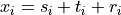
where i refers to a time index and the  term is used to quantify the trend and low-frequency variations
in the time series, the
term is used to quantify the trend and low-frequency variations
in the time series, the  term describes the harmonic component (e.g., diurnal or seasonal cycle) and
its modulation through time and, finally, the
term describes the harmonic component (e.g., diurnal or seasonal cycle) and
its modulation through time and, finally, the  term contains the residual component.
All the terms are estimated through a sequence of applications of locally weighted regression or low-order polynomial (e.g., LOESS) to data windows whose length is chosen by the user [Cleveland:1979] [Cleveland_Devlin:1988] [Cleveland_etal:1990].
Also included, are easy-to-use procedures for extracting frequency-defined series components from (multi-channel) time series based on the Fourier decomposition, which views the signal as a linear combination of purely harmonic components, each having a time-invariant amplitude and a well-defined frequency [Bloomfield:1976] [Duchon:1979] [Iacobucci_Noullez:2005].
These frequency filters can be obtained:
by windowing [Oppenheim_Schafer:1999]., which consists of convolving a specific window (such as a raised-cosine or Hamming/Hanning window) with the ideal rectangular filter response function in the frequency domain and using the FFT to transform from the time and frequency domains for the application of the windowed filter to the signal (see the
hwfilter()routine for example);by operating only in the time domain and using a moving data window which is centered on
 -th sample for extracting the desired
frequency component at the observation of the time series.
-th sample for extracting the desired
frequency component at the observation of the time series.
Here,
 is a non-negative integer called the window half-length, which
represents the number of samples before and after sample .
The total window length, which is also the number of filter coefficients to compute, is
is a non-negative integer called the window half-length, which
represents the number of samples before and after sample .
The total window length, which is also the number of filter coefficients to compute, is  .
.Routines are then provided to compute the symmetric linear filter coefficients with the user-desired properties (e.g., low-pass, band-pass or high-pass) in a first step [Bloomfield:1976] [Duchon:1979]. See the
lp_coef(),lp_coef2(),hp_coef(),hp_coef2(),bd_coef()andbd_coef2()routines for more details. These symmetric linear filter coefficients can then be applied to the signal in the time (or frequency) domain at the user option for performing the symmetric filtering operation of the time series in a second step (see thesymlin_filter()andsymlin_filter2()routines for example).
Finally, a large set of routines for spectral and cross-spectral estimations based on the FFT and smoothing the periodogram of time series in a variety of ways are also provided, see [Bloomfield:1976], [Welch:1967] and [Cooley_etal:1970], as well as a large variety of procedures for testing the hypothesis that two or several independent time-series are realizations of the same stationary process based on statistic computed from spectral density estimates of the time series [Diggle:1990].
Please note that routines provided in this module apply only to real data of kind stnd. The real kind type stnd is defined in module Select_Parameters.
In order to use one of these routines, you must include an appropriate use Time_Series_Procedures or use Statpack statement
in your Fortran program, like:
use Time_Series_Procedures, only: comp_smooth
or:
use Statpack, only: comp_smooth
Here is the list of the public routines exported by module Time_Series_Procedures:
-
comp_smooth()
Purpose:
comp_smooth() smooths a time series or a multichannel time series given in the argument X.
The smoothing is equivalent to the application of a moving average of approximately (2 * smooth_factor) + 1,
where smooth_factor is specified with the help of the input SMOOTH_FACTOR argument.
For more details, see [Olagnon:1996].
Synopsis:
call comp_smooth( x(:)     , smooth_factor                 )
call comp_smooth( x(:,:)   , smooth_factor , dimvar=dimvar )
call comp_smooth( x(:,:,:) , smooth_factor                 )
-
comp_trend()
Purpose:
comp_trend() extracts a smoothed component from a time series or a multichannel time series using a LOESS smoother [Cleveland:1979] [Cleveland_Devlin:1988].
In the LOESS procedure, the analyzed (multi-channel) time series is decomposed into two terms:
where i refers to a time index and the term is used to quantify the trend and low-frequency variations
in the time series and the term contains the residual component.
The trend is estimated through a sequence of applications of locally weighted regression or low-order
polynomial (e.g., a LOESS smoother) to data windows whose length is chosen by the user. More precisely, at each point  locally weighted regression is used to smooth the time series and find the trend
  . is the
the value at of a polynomial fit to the data using weighted least squares, where the weight for
. is the
the value at of a polynomial fit to the data using weighted least squares, where the weight for  is large
if is closed to
is large
if is closed to  and small if it is not.
The LOESS smoother for estimating the trend is specified with three parameters: a width (e.g., argument NT), a degree (e.g., argument ITDEG) and a jump (e.g., argument NTJUMP). The width specifies the number of data points that the local interpolation uses to smooth each point in the time series, the degree specifies the degree of the local polynomial that is fit to the data, and the jump specifies how many points are skipped between LOESS interpolations, with linear interpolation being done between these points.
If the optional ROBUST argument is set to true, the process is iterative and includes robustness
iterations that take advantages of the weighted-least-squares underpinnings of LOESS to remove the
effects of outliers [Cleveland:1979] [Cleveland_Devlin:1988].
comp_trend() returns the smoothed component (e.g., the trend) and, optionally, the robustness weights.
The input argument Y can be a time series (e.g., a vector) or a multichannel time series (e.g., a matrix and each column is a time series).
This subroutine is adapted from subroutine STL (Seasonal-Trend decomposition based on LOESS)
developed by Cleveland and coworkers at AT&T Bell Laboratories [Cleveland_etal:1990].
But, comp_trend() assumes that the time series has no seasonal cycle or other harmonic components.
If your time series include a seasonal cycle or other harmonic components, you must use comp_stl()
or comp_stlez() instead.
Note, finally, that comp_trend() expects equally spaced data with no missing values.
Synopsis:
call comp_trend( y(:n)    , nt , itdeg , robust , trend(:n)    , ntjump=ntjump , maxiter=maxiter , rw=rw , no=no , ok=ok )
call comp_trend( y(:n,:p) , nt , itdeg , robust , trend(:n,:p) , ntjump=ntjump , maxiter=maxiter , rw=rw , no=no , ok=ok )
-
comp_stlez()
Purpose:
comp_stlez() decomposes a time series vector or the (time series) columns of a matrix into seasonal and trend components using a Seasonal-Trend decomposition based on LOESS (STL) [Cleveland_etal:1990]. In the STL procedure, the analyzed (multi-channel) time series is decomposed into three terms:
where i refers to a time index and the term is used to quantify the trend and low-frequency variations
in the time series, the term describes the harmonic component (e.g., diurnal or seasonal cycle) and
its modulation through time and, finally, the term contains the residual component.
All the terms are estimated through a sequence of applications of locally weighted regression or low-order polynomial (e.g., LOESS)
to data windows whose length is chosen by the user [Cleveland:1979] [Cleveland_Devlin:1988]. This process is iterative with many steps
and may include robustness iterations (when the argument ROBUST is set to true) that take advantage of the weighted-least-squares
underpinnings of LOESS to remove the effects of outliers [Cleveland_etal:1990].
There are three LOESS smoothers in the process and each require three parameters: a width, a degree, and a jump. The width specifies the number of data points that the local interpolation uses to smooth each point, the degree specifies the degree of the local polynomial that is fit to the data, and the jump specifies how many points are skipped between LOESS interpolations, with linear interpolation being done between these points.
The LOESS smoother for estimating the trend is specified with the following parameters: a width (e.g., NT), a degree (e.g., ITDEG) and a jump (e.g., NTJUMP).
The LOESS smoother for estimating the seasonal component is specified with the following parameters: a width (e.g., NS), a degree (e.g., ISDEG) and a jump (e.g., NSJUMP).
The LOESS smoother for low-pass filtering is specified with the following parameters: a width (e.g., NL), a degree (e.g., ILDEG) and a jump (e.g., NLJUMP).
comp_stlez() is an iterative process, which may be interpreted as a frequency filter directly applicable to non-stationary (uni-dimensional) time series including harmonic components [Cleveland_etal:1990].
It returns the components and, optionally, the robustness weights.
This subroutine is a FORTRAN 90 implementation of subroutine STLEZ developed by Cleveland and coworkers at AT&T Bell Laboratories [Cleveland_etal:1990].
comp_stlez() offers an easy to use version of comp_stl() subroutine, also
included in STATPACK, by defaulting most parameters values associated
with the three LOESS smoothers described above and also used in comp_stl().
At a minimum, comp_stlez() requires specifying:
- the periodicity of the data (e.g., the NP argument,
12for monthly), - the width of the LOESS smoother used to smooth the cyclic seasonal sub-series (e.g., the NS argument),
- the degree of the locally-fitted polynomial in seasonal smoothing (e.g., ISDEG argument),
- the degree of the locally-fitted polynomial in trend smoothing (e.g., ITDEG argument).
comp_stlez() sets, by default, others parameters of the STL procedure to the values recommended
in [Cleveland_etal:1990] . It also includes tests of convergence if robust iterations
are carried out. Otherwise, comp_stlez() is similar to comp_stl().
If your time series do not include a seasonal cycle or other harmonic components, you must
use comp_trend() instead of comp_stlez().
Note, finally, that comp_stlez() expects equally spaced data with no missing values.
Synopsis:
call comp_stlez( y(:n)    , np , ns , isdeg , itdeg , robust , season(:n)    , trend(:n)    , ni=ni , nt=nt , nl=nl , ildeg=ildeg , nsjump=nsjump , ntjump=ntjump , nljump=nljump , maxiter=maxiter , rw=rw , no=no , ok=ok )
call comp_stlez( y(:n,:p) , np , ns , isdeg , itdeg , robust , season(:n,:p) , trend(:n,:p) , ni=ni , nt=nt , nl=nl , ildeg=ildeg , nsjump=nsjump , ntjump=ntjump , nljump=nljump , maxiter=maxiter , rw=rw , no=no , ok=ok )
-
comp_stl()
Purpose:
comp_stl() decomposes a time series vector or the (time series) columns of a matrix into seasonal and trend components using a Seasonal-Trend decomposition based on LOESS (STL) [Cleveland_etal:1990]. In the STL procedure, the analyzed (multi-channel) time series is decomposed into three terms:
where i refers to a time index and the term is used to quantify the trend and low-frequency variations
in the time series, the term describes the harmonic component (e.g., diurnal or seasonal cycle) and
its modulation through time and, finally, the term contains the residual component.
All the terms are estimated through a sequence of applications of locally weighted regression or low-order polynomial (e.g., LOESS)
to data windows whose length is chosen by the user [Cleveland:1979] [Cleveland_Devlin:1988]. This process is iterative with many steps
and may include robustness iterations (when the argument NO is set to an integer value greater than 0) that take advantage of
the weighted-least-squares underpinnings of LOESS to remove the effects of outliers [Cleveland_etal:1990].
There are three LOESS smoothers in the process and each require three parameters: a width, a degree, and a jump. The width specifies the number of data points that the local interpolation uses to smooth each point, the degree specifies the degree of the local polynomial that is fit to the data, and the jump specifies how many points are skipped between LOESS interpolations, with linear interpolation being done between these points.
The LOESS smoother for estimating the trend is specified with the following parameters: a width (e.g., NT), a degree (e.g., ITDEG) and a jump (e.g., NTJUMP).
The LOESS smoother for estimating the seasonal component is specified with the following parameters: a width (e.g., NS), a degree (e.g., ISDEG) and a jump (e.g., NSJUMP).
The LOESS smoother for low-pass filtering is specified with the following parameters: a width (e.g., NL), a degree (e.g., ILDEG) and a jump (e.g., NLJUMP).
comp_stl() is an iterative process, which may be interpreted as a frequency filter directly applicable to non-stationary (uni-dimensional) time series including harmonic components [Cleveland_etal:1990].
It returns the components and, optionally, the robustness weights.
This subroutine is a FORTRAN 90 implementation of subroutine STL developed by Cleveland and coworkers at AT&T Bell Laboratories [Cleveland_etal:1990].
If your time series do not include a seasonal cycle or other harmonic components, you must
use comp_trend() instead of comp_stl(). Also, if you don’t know how or want to specify
all the parameters in comp_stl(), you can use comp_stlez(), which is an easy to use
version of comp_stl().
Note, finally, that comp_stl() expects equally spaced data with no missing values.
Synopsis:
call comp_stl( y(:n)    , np , ni , no , isdeg , itdeg , ildeg , nsjump , ntjump , nljump , ns , nt , nl , rw , season(:n)    , trend(:n)    )
call comp_stl( y(:n,:p) , np , ni , no , isdeg , itdeg , ildeg , nsjump , ntjump , nljump , ns , nt , nl , rw , season(:n,:p) , trend(:n,:p) )
-
ma()
Purpose:
ma() smooths the vector X with a moving average of length LEN and output the result in the vector AVE.
This subroutine is a low-level subroutine used by subroutines comp_stlez() and comp_stl().
Synopsis:
call ma( x(:n) , len , ave(:n) )
-
detrend()
Purpose:
detrend() detrends a time series (e.g., the argument VEC) or a multi-channel time series (e.g., the rows of the matrix argument MAT).
If:
TREND =
1The mean of the time series is removedTREND =
2The drifts from the time series are estimated and removed by using the formula (for a time series):slope = (VEC(size(VEC)) - VEC(1))/(size(VEC) - 1)or (for a multi-channel time series):
slope(:) = (MAT(:,size(MAT,2)) - MAT(:,1))/(size(MAT,2) - 1)TREND =
3The least-squares lines from the time series are removed.
On exit, the original time series may be recovered with the formula (for a time series):
VEC(i) = VEC(i) + ORIG + SLOPE * real(i-1,stnd)
for i = 1, size(vec), or (for a multi-channel time series):
MAT(j,i) = MAT(j,i) + ORIG(j) + SLOPE(j) * real(i-1,stnd)
for i = 1, size(MAT,2) and j = 1, size(MAT,1), in all the cases.
Synopsis:
call detrend( vec(:n)    , trend , orig=orig ,     slope=slope     )
call detrend( vec(:p,:n) , trend , orig=orig(:p) , slope=slope(:p) )
-
hwfilter()
Purpose:
hwfilter() filters a time series (e.g., the vector argument VEC) or a multi-channel time series (e.g., the columns of the matrix argument MAT) in the frequency band limited by periods PL and PH by Hamming/Hanning-windowed (HW) filtering and a Fast Fourier Transform algorithm [Iacobucci_Noullez:2005].
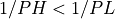
PL and PH are expressed in number of points, i.e. PL = 6(18) and PH = 32(96)
selects periods between 1.5 yrs and 8 yrs for quarterly (monthly) data, as an illustration.
Use PL = 0 for high-pass filtering frequencies corresponding to periods shorter than PH,
or PH = 0 for low-pass filtering frequencies corresponding to periods longer than PL.
Setting PH < PL is also allowed and performs band rejection of periods between PH and PL (i.e. in that case the meaning of the PL and PH arguments are reversed).
The frequency filter implemented in hwfilter() is obtained by convolving a raised-cosine window with the ideal rectangular filter response function. This windowed filter has almost no leakage and has a very flat response in the pass-band. Moreover, this filter is stationary and symmetric and, therefore, it induces no phase-shift. It is thus a good filter for extracting frequency-defined series components for short-length time series.
For more details, see [Iacobucci_Noullez:2005].
Synopsis:
call hwfilter( vec(:)   , pl , ph , initfft=initfft , trend=trend , win=win                       )
call hwfilter( mat(:,:) , pl , ph , initfft=initfft , trend=trend , win=win , max_alloc=max_alloc )
Examples:
-
hwfilter2()
Purpose:
hwfilter2() filters a time series (e.g., the vector argument VEC) or a multi-channel time series (e.g., the columns of the matrix argument MAT) in the frequency band limited by periods PL and PH by Hamming/Hanning-windowed (HW) filtering [Iacobucci_Noullez:2005].
PL and PH are expressed in number of points, i.e. PL = 6(18) and PH = 32(96)
selects periods between 1.5 yrs and 8 yrs for quarterly (monthly) data, as an illustration.
Use PL = 0 for high-pass filtering frequencies corresponding to periods shorter than PH,
or PH = 0 for low-pass filtering frequencies corresponding to periods longer than PL.
Setting PH < PL is also allowed and performs band rejection of periods between PH and PL (i.e. in that case the meaning of the PL and PH arguments are reversed).
The frequency filter implemented in hwfilter2() is obtained by convolving a raised-cosine window with the ideal rectangular filter response function. This windowed filter has almost no leakage and has a very flat response in the pass-band. Moreover, this filter is stationary and symmetric and, therefore, it induces no phase-shift. It is thus a good filter for extracting frequency-defined series components for short-length time series.
The unique difference between hwfilter2() and hwfilter() is the use of the Goertzel method
for computing the Fourier transform of the data (as in [Iacobucci_Noullez:2005]) instead of a Fast
Fourier Transform algorithm.
For more details, see [Iacobucci_Noullez:2005].
Synopsis:
call hwfilter2( vec(:)   , pl , ph , trend=trend , win=win )
call hwfilter2( mat(:,:) , pl , ph , trend=trend , win=win )
Examples:
-
lp_coef()
Purpose:
lp_coef() computes the K-term least squares approximation to an
-ideal- low pass filter with cutoff period PL (e.g., cutoff frequency  ).
).
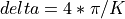
This filter has a transfer function with a transition band of width delta surrounding FC
equals to
when FC is expressed in radians.
lp_coef() computes symmetric linear low-pass filter coefficients using a least squares approximation to an ideal low-pass filter with convergence factors (i.e. a Lanczos window) which reduce overshoot and ripple [Bloomfield:1976].
This low-pass filter has a transfer function which changes from approximately
one to zero in a transition band about the ideal cutoff frequency FC (),
that is from  to
to  , as discussed in section 6.4 of
[Bloomfield:1976].
, as discussed in section 6.4 of
[Bloomfield:1976].
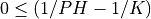
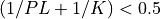
The user must specify the cutoff period (or the cutoff frequency) and the number of filter coefficients, which must be odd.
The user must also choose the number of filter coefficients, K, so that
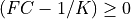 and
and 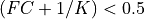 if the optional logical
argument NOTEST_FC is not used or is not set to
if the optional logical
argument NOTEST_FC is not used or is not set to true.
In addition, K must be chosen as a compromise between:
- a sharp cutoff, that is,
 small;
 - and minimizing the number of data points lost by the filtering operations
(e.g.,
 data points will be lost from each end of the series).
The subroutine returns the normalized low-pass filter coefficients.
For more details and algorithm, see Chapter 6 of [Bloomfield:1976].
Synopsis:
coef(:k) = lp_coef( pl , k , fc=fc , notest_fc=notest_fc )
Examples:
-
lp_coef2()
Purpose:
lp_coef2() computes the K-term least squares approximation to an
-ideal- low pass filter with cutoff period PL (e.g., cutoff frequency )
by windowed filtering (e.g., Hamming window is used).
This filter has a transfer function with a transition band of width delta surrounding FC
equals to
when FC is expressed in radians.
lp_coef2() computes symmetric linear low-pass filter coefficients using a least squares approximation to an ideal low-pass filter. The Hamming window is used to reduce overshoot and ripple in the transfer function of the ideal low-pass filter [Bloomfield:1976].
This low-pass filter has a transfer function which changes from approximately
one to zero in a transition band about the ideal cutoff frequency FC (),
that is from to , as discussed in section 6.4 of
[Bloomfield:1976].
The user must specify the cutoff period (or the cutoff frequency) and the number of filter coefficients, which must be odd.
The user must also choose the number of filter coefficients, K, so that
and if the optional logical
argument NOTEST_FC is not used or is not set to true.
The overshoot and the associated ripples in the ideal transfer function are reduced by the use of the Hamming window.
In addition, K must be chosen as a compromise between:
- a sharp cutoff, that is, small;
- and minimizing the number of data points lost by the filtering operations
(e.g., data points will be lost from each end of the series).
The subroutine returns the normalized low-pass filter coefficients.
For more details and algorithm, see Chapter 6 of [Bloomfield:1976].
Synopsis:
coef(:k) = lp_coef2( pl , k , fc=fc , win=win , notest_fc=notest_fc )
Examples:
-
hp_coef()
Purpose:
hp_coef() computes the K-term least squares approximation to an
-ideal- high pass filter with cutoff period PH (e.g., cutoff frequency 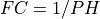 ).
).
This filter has a transfer function with a transition band of width delta surrounding FC
equals to
when FC is expressed in radians.
hp_coef() computes symmetric linear high-pass filter coefficients
from the corresponding low-pass filter as given by function lp_coef().
This is equivalent to subtracting the low-pass filtered series from the original
time series.
This high-pass filter has a transfer function which changes from approximately
zero to one in a transition band about the ideal cutoff frequency FC (),
that is from to , as discussed in section 6.4 of
[Bloomfield:1976].
The user must specify the cutoff period (or the cutoff frequency) and the number of filter coefficients, which must be odd.
The user must also choose the number of filter coefficients, K, so that
and if the optional logical
argument NOTEST_FC is not used or is not set to true.
In addition, K must be chosen as a compromise between:
- a sharp cutoff, that is, small;
- and minimizing the number of data points lost by the filtering operations
(e.g., data points will be lost from each end of the series).
The subroutine returns the high-pass filter coefficients.
For more details and algorithm, see Chapter 6 of [Bloomfield:1976].
Synopsis:
coef(:k) = hp_coef( ph , k , fc=fc , notest_fc=notest_fc )
Examples:
-
hp_coef2()
Purpose:
hp_coef2() computes the K-term least squares approximation to an
-ideal- high pass filter with cutoff period PH (e.g., cutoff frequency )
by windowed filtering (e.g., Hamming window is used).
This filter has a transfer function with a transition band of width delta surrounding FC
equals to
when FC is expressed in radians.
hp_coef() computes symmetric linear high-pass filter coefficients
from the corresponding low-pass filter as given by function lp_coef2().
This is equivalent to subtracting the low-pass filtered series from the original
time series.
This high-pass filter has a transfer function which changes from approximately
zero to one in a transition band about the ideal cutoff frequency FC (),
that is from to , as discussed in section 6.4 of
[Bloomfield:1976].
The user must specify the cutoff period (or the cutoff frequency) and the number of filter coefficients, which must be odd.
The user must also choose the number of filter coefficients, K, so that
and if the optional logical
argument NOTEST_FC is not used or is not set to true.
The overshoot and the associated ripples in the ideal transfer function are reduced by the use of the Hamming window.
In addition, K must be chosen as a compromise between:
- a sharp cutoff, that is, small;
- and minimizing the number of data points lost by the filtering operations
(e.g., data points will be lost from each end of the series).
The subroutine returns the high-pass filter coefficients.
For more details and algorithm, see Chapter 6 of [Bloomfield:1976].
Synopsis:
coef(:k) = hp_coef2( ph , k , fc=fc , win=win , notest_fc=notest_fc )
Examples:
-
bd_coef()
Purpose:
bd_coef() computes the K-term least squares approximation to an
-ideal- band pass filter with cutoff periods PL and PH (e.g., cutoff frequencies
 and
and  , respectively).
PL and PH are expressed in number of points, i.e. PL = 6(18) and PH = 32(96)
selects periods between 1.5 yrs and 8 yrs for quarterly (monthly) data, as an illustration.
Alternatively, the user can directly specify the two cutoff frequencies, FCL and FCH, corresponding to PL and PH.
bd_coef() computes symmetric linear band-pass filter coefficients using a least squares approximation to an ideal band-pass filter that has convergence factors which reduce overshoot and ripple [Bloomfield:1976].
This band-pass filter is computed as the difference between two low-pass filters
with cutoff frequencies and , respectively (or FCH and FCL).
This band-pass filter has a transfer function which changes from approximately
zero to one and one to zero in the transition bands about the ideal cutoff frequencies
and ), that is from 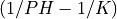 to
to 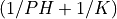 and
and 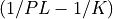 to
to 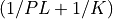 , respectively.
The user must specify the two cutoff periods and the number of filter coefficients, which must be odd.
The user must also choose the number of filter terms, K, so that:

However, if the optional logical argument NOTEST_FC is used and is set to true, the two tests
are bypassed.
In addition, K must be chosen as a compromise between:
- a sharp cutoff, that is, small;
- and minimizing the number of data points lost by the filtering operations
(e.g., data points will be lost from each end of the series).
The subroutine returns the difference between the two corresponding normalized low-pass filter coefficients
as computed by function lp_coef().
For more details and algorithm, see Chapter 6 of [Bloomfield:1976] and [Duchon:1979].
Synopsis:
coef(:k) = bd_coef( pl , ph , k , fch=fch , fcl=fcl , notest_fc=notest_fc )
Examples:
-
bd_coef2()
Purpose:
bd_coef2() computes the K-term least squares approximation to an
-ideal- band pass filter with cutoff periods PL and PH (e.g., cutoff frequencies
and , respectively) by windowed filtering (e.g., Hamming window is used)
[Bloomfield:1976].
PL and PH are expressed in number of points, i.e. PL = 6(18) and PH = 32(96)
selects periods between 1.5 yrs and 8 yrs for quarterly (monthly) data, as an illustration.
Alternatively, the user can directly specify the two cutoff frequencies, FCL and FCH, corresponding to PL and PH.
bd_coef2() computes symmetric linear band-pass filter coefficients using a least squares approximation to an ideal band-pass filter. The Hamming window is used to reduce overshoot and ripple in the transfer function of the ideal low-pass filter.
This band-pass filter is computed as the difference between two low-pass filters
with cutoff frequencies and , respectively (or FCH and FCL).
This band-pass filter has a transfer function which changes from approximately
zero to one and one to zero in the transition bands about the ideal cutoff frequencies
and ), that is from to and
to , respectively.
The user must specify the two cutoff periods and the number of filter coefficients, which must be odd.
The user must also choose the number of filter terms, K, so that:
However, if the optional logical argument NOTEST_FC is used and is set to true, the two tests
are bypassed.
The overshoot and the associated ripples in the ideal transfer function are reduced by the use of the Hamming window.
In addition, K must be chosen as a compromise between:
- a sharp cutoff, that is, small;
- and minimizing the number of data points lost by the filtering operations
(e.g., data points will be lost from each end of the series).
The subroutine returns the difference between the two corresponding normalized low-pass filter coefficients
as computed by function lp_coef2().
For more details and algorithm, see Chapter 6 of [Bloomfield:1976].
Synopsis:
coef(:k) = bd_coef2( pl , ph , k , fch=fch , fcl=fcl , win=win , notest_fc=notest_fc )
Examples:
-
pk_coef()
Purpose:
pk_coef() computes the K-term least squares approximation to an
-ideal- band pass filter with peak response near one at the single frequency
FREQ (e.g., the peak response is at  ).
).
pk_coef() computes symmetric linear band-pass filter coefficients using a least squares approximation to an ideal band-pass filter that has convergence factors which reduce overshoot and ripple [Bloomfield:1976].
This band-pass filter is computed as the difference between two low-pass filters
with cutoff frequencies FCL and FCH, respectively. See [Duchon:1979] for the
computations of the two cutoff frequencies FCL and FCH.
This band-pass filter has a transfer function which changes from approximately
zero to one and one to zero in the transition bands about the cutoff frequencies FCH and FCL,
that is from  to FREQ and FREQ to
  , respectively.
The user must specify the frequency FREQ with unit response and the number of filter coefficients, K, which must be odd. The user must also choose the number of filter terms, K, as a compromise between:
- a sharp cutoff, that is, small;
- and minimizing the number of data points lost by the filtering operations
(e.g., data points will be lost from each end of the series).
The subroutine returns the difference between the two corresponding normalized low-pass filter coefficients
as computed by function lp_coef().
For more details and algorithm, see Chapter 6 of [Bloomfield:1976] and [Duchon:1979].
Synopsis:
coef(:k) = pk_coef( freq , k , notest_freq=notest_freq )
Examples:
-
moddan_coef()
Purpose:
moddan_coef() computes the impulse response function (e.g., weights) corresponding to a number
of applications of modified Daniell filters as done in subroutine moddan_filter().
For definition, more details and algorithm, see [Bloomfield:1976].
Synopsis:
coef(:k) = moddan_coef( k , smooth_param(:) )
-
freq_func()
Purpose:
freq_func() computes the frequency response function (e.g., the transfer function) of the symmetric linear filter given by the argument COEF(:).
The frequency response function is computed at NFREQ frequencies regularly sampled
between zero and the Nyquist frequency if the optional logical argument FOUR_FREQ is not used
or at the NFREQ Fourier frequencies 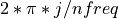 for j =
  to
to  if this argument is used and set to
 true.
For more details, see [Bloomfield:1976] and [Oppenheim_Schafer:1999].
Synopsis:
call freq_func( nfreq , coef(:) , freqr(:nfreq) , four_freq=four_freq , freq=freq(:nfreq) )
Examples:
-
symlin_filter()
Purpose:
symlin_filter() performs a symmetric filtering operation on an input time series (e.g., the vector argument VEC) or multi-channel time series (e.g., the matrix argument MAT).
The filtering is done in place and (size(COEF)-1)/2 observations will be lost from
each end of the (multi-channel) time series.
Note, also, that the filtered (multi-channel) time series is shifted in time and is stored on output in:
VEC(1:NFILT), with NFILT =size(VEC) - size(COEF) + 1.MAT(:,1:NFILT), with NFILT =size(MAT,2) - size(COEF) + 1.
The symmetric linear filter coefficients (e.g., the array COEF) can be computed with
the help of functions lp_coef, lp_coef2, hp_coef, hp_coef2,
bd_coef and bd_coef2.
Synopsis:
call symlin_filter( vec(:)   , coef(:) , trend=trend , nfilt=nfilt )
call symlin_filter( mat(:,:) , coef(:) , trend=trend , nfilt=nfilt )
Examples:
-
symlin_filter2()
Purpose:
symlin_filter2() performs a symmetric filtering operation on an input time series (e.g., the vector argument VEC) or multi-channel time series (e.g., the matrix argument MAT).
No time observations will be lost, however the first and last (size(COEF)-1)/2 time
observations are affected by end effects.
If USEFFT is used with the value true, the values at both ends of the output (multi-channel) series
are computed by assuming that the input (multi-channel) series is part of a periodic sequence of
period size(VEC) (or size(MAT,2). Otherwise, each end of the filtered (multi-channel)time series
is estimated by truncated the symmetric linear filter coefficients array COEF(:).
The symmetric linear filter coefficients (e.g., the array COEF) can be computed with
the help of functions lp_coef, lp_coef2, hp_coef, hp_coef2,
bd_coef and bd_coef2.
Synopsis:
call symlin_filter2( vec(:)   , coef(:) , trend=trend , usefft=usefft , initfft=initfft )
call symlin_filter2( mat(:,:) , coef(:) , trend=trend , usefft=usefft , initfft=initfft )
Examples:
-
dan_filter()
Purpose:
dan_filter() smooths an input time series (e.g., the vector argument VEC) or multi-channel time series (e.g., the matrix argument MAT) by applying a Daniell filter (e.g., a simple moving average) of length NSMOOTH.
dan_filter() smooths an input (multi-channel) time series by applying a Daniell filter as discussed in chapter 7 of [Bloomfield:1976].
This subroutine use the hypothesis of an (even or odd) symmetry of the input (multi-channel) time series to avoid losing values from the ends of the series.
For more details and algorithm, see chapter 7 of [Bloomfield:1976].
Synopsis:
call dan_filter( vec(:)   , nsmooth , sym=sym , trend=trend )
call dan_filter( mat(:,:) , nsmooth , sym=sym , trend=trend )
-
moddan_filter()
Purpose:
moddan_filter() smooths an input time series (e.g., the vector argument VEC) or multi-channel time series (e.g., the matrix argument MAT) by applying a sequence of modified Daniell filters.
moddan_filter() smooths an input (multi-channel) time series by applying a sequence of modified Daniell filters as discussed in chapter 7 of [Bloomfield:1976]. This subroutine use the hypothesis of an (even or odd) symmetry of the input time series to avoid losing values from the ends of the series.
For more details and algorithm, see chapter 7 of [Bloomfield:1976].
Synopsis:
call moddan_filter( vec(:)   , smooth_param(:) , sym=sym , trend=trend )
call moddan_filter( mat(:,:) , smooth_param(:) , sym=sym , trend=trend )
-
extend()
Purpose:
extend() returns the INDEX-th term in the time series VEC or the multi-channel time series MAT, extending it if necessary with an even or odd symmetry according to the sign of SYM, which should be either plus or minus one. Note also that the value zero will result in the extended value being zero.
For more details and algorithm, see Chapter 6 of [Bloomfield:1976].
Synopsis:
x     = extend( vec(:p)    , index , sym )
x(:n) = extend( mat(:n,:p) , index , sym )
-
taper()
Purpose:
taper() applies a split-cosine-bell taper on an input time series VEC or a multi-channel time series MAT.
This subroutine is adapted from Chapter 5 of [Bloomfield:1976].
Synopsis:
call taper( vec(:)   , taperp )
call taper( mat(:,:) , taperp )
-
data_window()
Purpose:
data_window() computes data windows used in spectral computations.
For more details, see Chapter 5 of [Bloomfield:1976].
Synopsis:
wk(:n) = data_window( n , win , taperp=taperp )
-
estim_dof()
Purpose:
estim_dof() computes the equivalent number of degrees of freedom of power
and cross spectrum estimates as calculated by subroutines power_spectrum(),
cross_spectrum(), power_spectrum2() and cross_spectrum2().
The computed equivalent number of degrees of freedom must be divided by two for the zero and Nyquist frequencies.
Furthermore, the computed equivalent number of degrees of freedom is not right near the zero and Nyquist frequencies if the Power Spectral Density (PSD) estimates have been smoothed by modified Daniell filters.
The reason is that estim_dof() assumes that smoothing involves averaging independent frequency ordinates. This is true except near the zero and Nyquist frequencies where an average may contain contributions from negative frequencies, which are identical to and hence not independent of positive frequency spectral values. Thus, the number of degrees of freedom in PSD estimates near the zero and Nyquist frequencies are as little as half the number of degrees of freedom of the spectral estimates away from these frequency extremes if the optional argument SMOOTH_PARAM is used.
For more details and algorithm, see [Bloomfield:1976] and [Welch:1967].
Synopsis:
edof = estim_dof( wk(:n) , win=win , smooth_param=smooth_param , l0=l0 , nseg=nseg , overlap=overlap )
-
estim_dof2()
Purpose:
estim_dof2() computes the equivalent number of degrees of freedom of power
and cross spectrum estimates as calculated by subroutines power_spectrm(),
cross_spectrm(), power_spectrm2() and cross_spectrm2().
For more details and algorithm, see [Bloomfield:1976] and [Welch:1967].
Synopsis:
edof(:(n+l0)/2 + 1 ) = estim_dof2( wk(:n) , l0 , win=win , nsmooth=nsmooth , nseg=nseg , overlap=overlap )
-
comp_conflim()
Purpose:
comp_conflim() estimates confidence limit factors for spectral estimates and, optionally, critical values for testing the null hypothesis that the squared coherencies between two time series are zero.
Synopsis:
call comp_conflim( edof     , probtest=probtest , conlwr=conlwr     , conupr=conupr     , testcoher=testcoher     )
call comp_conflim( edof(:n) , probtest=probtest , conlwr=conlwr(:n) , conupr=conupr(:n) , testcoher=testcoher(:n) )
-
spctrm_ratio()
Purpose:
spctrm_ratio() calculates a point-wise tolerance intervals for the ratios of two estimated spectra under the assumption that the two “true” underlying spectra are the same.
For more details, see Chapter 4 of [Diggle:1990].
Synopsis:
call spctrm_ratio( edofn     , edofd     , lwr_ratio     , upr_ratio     , pinterval=pinterval )
call spctrm_ratio( edofn(:n) , edofd(:n) , lwr_ratio(:n) , upr_ratio(:n) , pinterval=pinterval )
-
spctrm_ratio2()
Purpose:
spctrm_ratio2() calculates a conservative critical probability values (e.g., p-values) for testing the hypothesis of a common spectrum for two estimated (multi-channel) spectra (e.g., the arguments PSVECN, PSVECD or PSMATN, PSMATD).
These conservative critical probability values are computed from the minimum and maximum values of the ratio of the two estimated (multichannel) spectra and the associated probabilities of obtaining, respectively, a value less (for the minimum ratios) and higher (for the maximum ratios) than attained under the null hypothesis of a common spectra for the two (multichannel) time series.
This statistical test relies on the assumptions that the different spectral ordinates have the same sampling distribution and are independent of each other for each series. This means, in particular, that the spectral ordinates corresponding to the zero and Nyquist frequencies must be excluded from the PSVECN and PSVECD vectors (or PSMATN, PSMATD matrices) before calling spctrm_ratio2() and that the two estimated (multi-channel) spectra have not been obtained by smoothing the periodograms in the frequency domain, but by averaging different periodograms computed on replicated time series.
It is also assumed that the (multichannel) time series with spectra PSVECN and PSVECD (or PSMATN and PSMATD) are independent realizations.
For more details, see Chapter 4 of [Diggle:1990].
Synopsis:
call spctrm_ratio2( psvecn(:n)    , psvecd(:n)    , edofn , edofd , prob     , min_ratio=min_ratio     , max_ratio=max_ratio    , prob_min_ratio=prob_min_ratio      , prob_max_ratio=prob_max_ratio     )
call spctrm_ratio2( psmatn(:p,:n) , psmatd(:p,:n) , edofn , edofd , prob(:p) , min_ratio=min_ratio(:p) , max_ratio=max_ratio(:p) , prob_min_ratio=prob_min_ratio(:p) , prob_max_ratio=prob_max_ratio(:p) )
-
spctrm_ratio3()
Purpose:
spctrm_ratio3() calculates approximate critical probability values (e.g., p-values) for testing the hypothesis of a common spectrum for two estimated (multi-channel) spectra (e.g., the vector arguments PSVECN, PSVECD or matrix arguments PSMATN, PSMATD). These approximate critical probability values are derived from the following chi-squared log-ratio statistics:

where
 =
= size(PSVECN)=size(PSVECD)
where
= size(PSMATN,2)=size(PSMATD,2)andn=size(PSMATN,1)=size(PSMATD,1)is the number of channels in the two multi-channel time series.
In both cases, is the number of frequencies considered. Arguments EDOFN and EDOFD give, respectively, the equivalent
numbers of degrees of freedom,  and
and  , of the first and second estimated spectra (e.g., the numerator and denominator
of the ratio of the two estimated spectra). These numbers can be computed by the
, of the first and second estimated spectra (e.g., the numerator and denominator
of the ratio of the two estimated spectra). These numbers can be computed by the estim_dof() and estim_dof2() functions.
In order to derive approximate critical probability values, it is assumed that  (or
(or  for i =
  to
to  ) has an approximate chi-squared distribution with degrees of
freedom:
) has an approximate chi-squared distribution with degrees of
freedom:  [Jenkins_Watts:1968] [Priestley:1981].
The chi-squared log-ratio statistics are stored on output in the CHI2_STAT scalar or vector arguments.
This statistical test relies on the assumptions that the different spectral ordinates have the same sampling distribution and are independent of each other for each time series. This means, in particular, that the spectral ordinates corresponding to the zero and Nyquist frequencies must be excluded from the PSVECN and PSVECD vector ( or PSMATN and PSMATD matrix) spectra before calling spctrm_ratio3() and that the two estimated (multi-channel) spectra have not been obtained by smoothing the periodogram in the frequency domain, but by averaging different periodograms computed on replicated time series.
Thus, this test could only be used to compare two periodograms or two spectral estimates computed as the the average of, say, r periodograms for each time series.
It is also assumed that the (multichannel) time series with spectra PSVECN and PSVECD (or PSMATN and PSMATD) are independent realizations.
Synopsis:
call spctrm_ratio3( psvecn(:n)    , psvecd(:n)    , edofn , edofd , chi2_stat     , prob     )
call spctrm_ratio3( psmatn(:p,:n) , psmatd(:p,:n) , edofn , edofd , chi2_stat(:p) , prob(:p) )
-
spctrm_ratio4()
Purpose:
spctrm_ratio4() calculates approximate critical probability values (e.g., p-values) for testing the hypothesis of a common shape for two estimated (multi-channel) spectra (e.g., the vector arguments PSVECN, PSVECD or matrix arguments PSMATN, PSMATD). These approximate critical probability values are derived from the following range log-ratio statistics:

where
= size(PSVECN)=size(PSVECD)
where
= size(PSMATN,2)=size(PSMATD,2)andn=size(PSMATN,1)=size(PSMATD,1)is the number of channels in the two multi-channel time series.
In both cases, is the number of frequencies considered. Arguments EDOFN and EDOFD give, respectively, the equivalent
numbers of degrees of freedom, and , of the first and second estimated spectra (e.g., the numerator and denominator
of the ratio of the two estimated spectra). These numbers can be computed by the estim_dof() and estim_dof2() functions.
In order to derive approximate critical probability values, it is assumed that the elements of the vector  (or of the vectors
  for i = to ) are independent and follow approximately a normal
distribution with mean
for i = to ) are independent and follow approximately a normal
distribution with mean 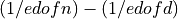 and variance
 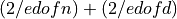 . In these conditions, the distribution of the
 statistics may be approximated by the distribution function of the range of independent normal random variables
(with mean and variance as specified above) as computed by the
statistics may be approximated by the distribution function of the range of independent normal random variables
(with mean and variance as specified above) as computed by the rangen() routine in the
Prob_Procedures module [Potscher_Reschenhofer:1989].
The range log-ratio statistics are stored on output in the RANGE scalar or vector arguments.
This statistical test relies on the assumptions that the different spectral ordinates have the same sampling distribution and are independent of each other for each time series. This means, in particular, that the spectral ordinates corresponding to the zero and Nyquist frequencies must be excluded from the PSVECN and PSVECD vector arguments (or from the PSMATN and PSMATD matrix arguments) before calling spctrm_ratio4() and that the two estimated spectra have not been obtained by smoothing the periodogram in the frequency domain, but by averaging different periodograms computed on replicated time series.
Thus, this test could only be used to compare two periodograms or two spectral estimates computed as the the average of, say, r periodograms for each time series.
It is also assumed that the (multichannel) time series with spectra PSVECN and PSVECD (or PSMATN and PSMATD) are independent realizations.
For more details and theory, see [Coates_Diggle:1986] [Potscher_Reschenhofer:1988] [Potscher_Reschenhofer:1989].
Synopsis:
call spctrm_ratio4( psvecn(:n)    , psvecd(:n)    , edofn , edofd , range_stat     , prob     )
call spctrm_ratio4( psmatn(:p,:n) , psmatd(:p,:n) , edofn , edofd , range_stat(:p) , prob(:p) )
-
spctrm_diff()
Purpose:
spctrm_diff() calculates approximate critical probability values (e.g., p-values) for testing the hypothesis of a common shape for two estimated (multi-channel) spectra (e.g., the vector arguments PSVEC1 and PSVEC2 or matrix arguments PSMAT1, PSMAT2). These approximate critical probability values are derived from the following Kolmogorov-Smirnov statistics (stored in the KS_STAT output scalar or vector arguments):

where
= size(PSVEC1)=size(PSVEC2) for
for  = to
= to where
= size(PSMAT1,2)=size(PSMAT2,2)andn=size(PSMAT1,1)=size(PSMAT2,1)is the number of channels in the two multi-channel time series.
In both cases, is the number of frequencies considered and F1() and F2() are the normalized cumulative periodograms
computed from the estimated spectra PSVEC1 and PSVEC2 (or PSMAT1 and PSMAT2).
The distribution of D under the null hypothesis of a common shape for the spectra of the two series is approximated by calculating D for some large number (e.g., the NREP argument) of random interchanges of periodogram ordinates at each frequency for the two estimated (multi-channel) spectra [Diggle_Fisher:1991].
This statistical randomization test relies on the assumptions that the different spectral ordinates have the same sampling distribution and are independent of each other [Priestley:1981]. This means, in particular, that the spectral ordinates corresponding to the zero and Nyquist frequencies must be excluded from the PSVEC1 and PSVEC2 vectors ( or the PSMAT1 and PSMAT2 matrices) before calling spctrm_diff() and that the two estimated multichannel spectra have not been obtained by smoothing the periodograms in the frequency domain.
Thus, this randomization test could only be used to compare two periodograms or two spectral estimates computed as the the average of, say, r periodograms for each time series.
For more details, see [Diggle_Fisher:1991].
Synopsis:
call spctrm_diff( psvec1(:n)    , psvec2(:n)    , ks_stat     , prob     , nrep=nrep , norm=norm , initseed=initseed )
call spctrm_diff( psmat1(:p,:n) , psmat2(:p,:n) , ks_stat(:p) , prob(:p) , nrep=nrep , norm=norm , initseed=initseed )
-
spctrm_diff2()
Purpose:
spctrm_diff2() calculates approximate critical probability values (e.g., p-values) for testing the hypothesis of a common underlying spectrum for the two estimated (multi-channel) spectra (e.g., the vector arguments PSVEC1 and PSVEC2 or matrix arguments PSMAT1, PSMAT2). These approximate critical probability values are derived from the following chi-squared log-ratio statistics (stored in the CHI2_STAT output scalar or vector arguments):

where
= size(PSVEC1)=size(PSVEC2)
where
= size(PSMAT1,2)=size(PSMAT2,2)andn=size(PSMAT1,1)=size(PSMAT2,1)is the number of channels in the two multi-channel time series.
In both cases, is the number of frequencies considered.
The distribution of the chi-squared statistics under the null hypothesis of a common spectrum for the spectra of the
two (multi-channel) time series is approximated by calculating the chi-squared statistic for some large number (e.g., the NREP
argument) of random interchanges of periodogram ordinates at each frequency for the two
estimated (multi-channel) spectra (e.g., the arguments PSVEC1 and PSVEC2 or PSMAT1 and PSMAT2).
This statistical randomization test relies on the assumptions that the different spectral ordinates have the same sampling distribution and are independent of each other [Priestley:1981]. This means, in particular, that the spectral ordinates corresponding to the zero and Nyquist frequencies must be excluded from the PSVEC1 and PSVEC2 vectors (or PSMAT1 and PSMAT2 matrices) before calling spctrm_dif2f() and that the two estimated (multi-channel) spectra have not been obtained by smoothing the periodograms in the frequency domain.
Thus, this randomization test could only be used to compare two periodograms or two spectral estimates computed as the the average of, say, r periodograms for each time series.
Finally, none of the spectral estimates must be zero.
For more details, see [Diggle_Fisher:1991].
Synopsis:
call spctrm_diff2( psvec1(:n)    , psvec2(:n)    , chi2_stat     , prob     , nrep=nrep , initseed=initseed )
call spctrm_diff2( psmat1(:p,:n) , psmat2(:p,:n) , chi2_stat(:p) , prob(:p) , nrep=nrep , initseed=initseed )
-
power_spctrm()
Purpose:
power_spctrm() computes Fast Fourier Transform (FFT) estimates of the power spectrum of a real (multi-channel) time series (e.g., the vector argument VEC or matrix argument MAT). The real valued sequence time series must be of even length in all cases.
The Power Spectral Density (PSD) estimates are returned in units which are
the square of the data (if NORMPSD = false) or in spectral density
units (if NORMPSD = true).
After removing the mean or the trend from the (multi-channel) time series (e.g., the TREND argument), the selected data window (e.g., the WIN argument) is applied to the (multi-channel) time series and the PSD estimates are computed by the FFT of this transformed (multi-channel) time series. Optionally, theses PSD estimates may then be smoothed in the frequency domain by a Daniell filter (e.g., if the NSMOOTH argument is used).
For definitions, more details and algorithm, see [Bloomfield:1976], [Welch:1967] [Cooley_etal:1970] and [Diggle:1990].
Synopsis:
call power_spctrm( vec(:n)    , psvec(:(n/2)+1)    , freq=freq(:(n/2)+1) , fftvec=fftvec(:(n/2)+1)    , edof=edof(:(n/2)+1) , bandwidth=bandwidth(:(n/2)+1) , conlwr=conlwr(:(n/2)+1) , conupr=conupr(:(n/2)+1) , initfft=initfft , normpsd=normpsd , nsmooth=nsmooth , trend=trend , win=win , taperp=taperp , probtest=probtest )
call power_spctrm( mat(:p,:n) , psmat(:p,:(n/2)+1) , freq=freq(:(n/2)+1) , fftmat=fftmat(:p,:(n/2)+1) , edof=edof(:(n/2)+1) , bandwidth=bandwidth(:(n/2)+1) , conlwr=conlwr(:(n/2)+1) , conupr=conupr(:(n/2)+1) , initfft=initfft , normpsd=normpsd , nsmooth=nsmooth , trend=trend , win=win , taperp=taperp , probtest=probtest )
-
cross_spctrm()
Purpose:
cross_spctrm() computes Fast Fourier Transform (FFT) estimates of the power and cross-spectra of two real time series (e.g., the vector arguments VEC and VEC2) or a real time series and a (multi-channel) time series (e.g., the vector argument *VEC and matrix argument MAT). The real valued sequence time series must be of even length in all cases.
The Power Spectral Density (PSD) and Cross Spectral Density (CSD) estimates are returned in units which are
the square of the data (if NORMPSD = false) or in spectral density units (if NORMPSD = true).
After removing the mean or the trend from the (multi-channel) time series (e.g., the TREND argument), the selected data window (e.g., the WIN argument) is applied to the (multi-channel) time series and the PSD and CSD estimates are computed by the FFT of this transformed (multi-channel) time series. Optionally, theses PSD estimates may then be smoothed in the frequency domain by a Daniell filter (e.g., if the NSMOOTH argument is used).
For definitions, more details and algorithm, see [Bloomfield:1976], [Welch:1967] [Cooley_etal:1970] and [Diggle:1990].
Synopsis:
call cross_spctrm( vec(:n) , vec2(:n)   , psvec(:(n/2)+1) , psvec2(:(n/2)+1)   , phase(:(n/2)+1)    , coher(:(n/2)+1)    , freq=freq(:(n/2)+1) , edof=edof(:(n/2)+1) , bandwidth=bandwidth(:(n/2)+1) , conlwr=conlwr(:(n/2)+1) , conupr=conupr(:(n/2)+1) , testcoher=testcoher(:(n/2)+1) , ampli=ampli(:(n/2)+1)    , co_spect=co_spect(:(n/2)+1)    , quad_spect=quad_spect(:(n/2)+1)    , prob_coher=prob_coher(:(n/2)+1)    , initfft=initfft , normpsd=normpsd , nsmooth=nsmooth , trend=trend , win=win , taperp=taperp , probtest=probtest )
call cross_spctrm( vec(:n) , mat(:p,:n) , psvec(:(n/2)+1) , psmat(:p,:(n/2)+1) , phase(:p,:(n/2)+1) , coher(:p,:(n/2)+1) , freq=freq(:(n/2)+1) , edof=edof(:(n/2)+1) , bandwidth=bandwidth(:(n/2)+1) , conlwr=conlwr(:(n/2)+1) , conupr=conupr(:(n/2)+1) , testcoher=testcoher(:(n/2)+1) , ampli=ampli(:p,:(n/2)+1) , co_spect=co_spect(:p,:(n/2)+1) , quad_spect=quad_spect(:p,:(n/2)+1) , prob_coher=prob_coher(:p,:(n/2)+1) , initfft=initfft , normpsd=normpsd , nsmooth=nsmooth , trend=trend , win=win , taperp=taperp , probtest=probtest )
-
power_spctrm2()
Purpose:
power_spctrm2() computes Fast Fourier Transform (FFT) estimates of the power spectrum of a real (multi-channel) time series (e.g., the vector argument VEC or matrix argument MAT).
The Power Spectral Density (PSD) estimates are returned in units which are
the square of the data (if NORMPSD = false) or in spectral density
units (if NORMPSD = true).
After removing the mean or the trend from the (multi-channel) time series (e.g., the TREND argument), the time series
are padded with zero on the right such that the length of the resulting augmented time series are
evenly divisible by L (a positive even integer). The length, say n, of this resulting (multi-channel) time
series is the first integer greater than or equal to size(VEC) (or size(MAT,2)) which is evenly divisible
by L. If size(VEC) (or size(MAT,2)) is not evenly divisible by L, n is equal to
size(VEC)+L-mod(size(VEC),L) (or size(MAT,2)+L-mod(size(MAT,2),L).
Once the (multi-channel) time series has been segmented, the mean or the trend may also be removed from each (multi-channel) time segment (e.g., the TREND2 argument), a data window (e.g., the WIN argument) is, eventually, applied to the (multi-channel) time segments. Optionally, zeros may also be added to each (multi-channel) time segment (e.g., the optional argument L0) if more finely spaced spectral estimates are desired [Welch:1967] [Cooley_etal:1970].
The PSD estimates are then derived by computing and averaging the FFTs of the transformed (multi-channel) time segments
(e.g., modified periodograms). The stability of the PSD estimates depends on the averaging process. That is, the greater
the number of segments ( n/L if OVERLAP = false and (2n/L)-1 if OVERLAP = true),
the more stable the resulting PSD estimates [Welch:1967] [Cooley_etal:1970].
Optionally, theses PSD estimates may then be smoothed again in the frequency domain by a Daniell filter (e.g., if the NSMOOTH argument is used).
For definitions, more details and algorithm, see [Bloomfield:1976], [Welch:1967] [Cooley_etal:1970] and [Diggle:1990].
Synopsis:
call power_spctrm2( vec(:n)    , l , psvec(:((l+l0)/2)+1)    , freq=freq(:((l+l0)/2)+1) , edof=edof(:((l+l0)/2)+1) , bandwidth=bandwidth(:((l+l0)/2)+1) , conlwr=conlwr(:((l+l0)/2)+1) , conupr=conupr(:((l+l0)/2)+1) , initfft=initfft , overlap=overlap , normpsd=normpsd , nsmooth=nsmooth , trend=trend , trend2=trend2 , win=win , taperp=taperp , l0=l0 , probtest=probtest )
call power_spctrm2( mat(:p,:n) , l , psmat(:p,:((l+l0)/2)+1) , freq=freq(:((l+l0)/2)+1) , edof=edof(:((l+l0)/2)+1) , bandwidth=bandwidth(:((l+l0)/2)+1) , conlwr=conlwr(:((l+l0)/2)+1) , conupr=conupr(:((l+l0)/2)+1) , initfft=initfft , overlap=overlap , normpsd=normpsd , nsmooth=nsmooth , trend=trend , trend2=trend2 , win=win , taperp=taperp , l0=l0 , probtest=probtest )
-
cross_spctrm2()
Purpose:
cross_spctrm2() computes Fast Fourier Transform (FFT) estimates of the power and cross-spectra of two real time series (e.g., the vector arguments VEC and VEC2) or a real time series and a (multi-channel) time series (e.g., the vector argument *VEC and matrix argument MAT).
The Power Spectral Density (PSD) and Cross Spectral Density (CSD) estimates are returned in units which are
the square of the data (if NORMPSD = false) or in spectral density
units (if NORMPSD = true).
After removing the mean or the trend from the (multi-channel) time series (e.g., the TREND argument), the time series
are padded with zero on the right such that the length of the resulting augmented time series are
evenly divisible by L (a positive even integer). The length, say n, of this resulting (multi-channel) time
series is the first integer greater than or equal to size(VEC) which is evenly divisible
by L. If size(VEC) is not evenly divisible by L, n is equal to size(VEC)+L-mod(size(VEC),L).
Once the (multi-channel) time series have been segmented, the mean or the trend may also be removed from each (multi-channel) time segment (e.g., the TREND2 argument), a data window (e.g., the WIN argument) is, eventually, applied to the (multi-channel) time segments. Optionally, zeros may also be added to each (multi-channel) time segment (e.g., the optional argument L0) if more finely spaced spectral estimates are desired [Welch:1967] [Cooley_etal:1970].
The PSD and CSD estimates are then derived by computing and averaging the FFTs of the transformed (multi-channel) time segments
(e.g., modified periodograms). The stability of the PSD and CSD estimates depends on the averaging process. That is, the greater
the number of segments ( n/L if OVERLAP = false and (2n/L)-1 if OVERLAP = true),
the more stable the resulting PSD estimates [Welch:1967] [Cooley_etal:1970].
Optionally, theses PSD and CSD estimates may then be smoothed again in the frequency domain by a Daniell filter (e.g., if the NSMOOTH argument is used).
For definitions, more details and algorithm, see [Bloomfield:1976], [Welch:1967] [Cooley_etal:1970] and [Diggle:1990].
Synopsis:
call cross_spctrm2( vec(:n) , vec2(:n)   , l , psvec(:((l+l0)/2)+1) , psvec2(:((l+l0)/2)+1)   , phase(:((l+l0)/2)+1)    , coher(:((l+l0)/2)+1)    , freq=freq(:((l+l0)/2)+1) , edof=edof(:((l+l0)/2)+1) , bandwidth=bandwidth(:((l+l0)/2)+1) , conlwr=conlwr(:((l+l0)/2)+1) , conupr=conupr(:((l+l0)/2)+1) , testcoher=testcoher(:((l+l0)/2)+1) , ampli=ampli(:((l+l0)/2)+1)    , co_spect=co_spect(:((l+l0)/2)+1)    , quad_spect=quad_spect(:((l+l0)/2)+1)    , prob_coher=prob_coher(:((l+l0)/2)+1)    , initfft=initfft , overlap=overlap , normpsd=normpsd , nsmooth=nsmooth , trend=trend , trend2=trend2 , win=win , taperp=taperp , l0=l0 , probtest=probtest )
call cross_spctrm2( vec(:n) , mat(:p,:n) , l , psvec(:((l+l0)/2)+1) , psmat(:p,:((l+l0)/2)+1) , phase(:p,:((l+l0)/2)+1) , coher(:p,:((l+l0)/2)+1) , freq=freq(:((l+l0)/2)+1) , edof=edof(:((l+l0)/2)+1) , bandwidth=bandwidth(:((l+l0)/2)+1) , conlwr=conlwr(:((l+l0)/2)+1) , conupr=conupr(:((l+l0)/2)+1) , testcoher=testcoher(:((l+l0)/2)+1) , ampli=ampli(:p,:((l+l0)/2)+1) , co_spect=co_spect(:p,:((l+l0)/2)+1) , quad_spect=quad_spect(:p,:((l+l0)/2)+1) , prob_coher=prob_coher(:p,:((l+l0)/2)+1) , initfft=initfft , overlap=overlap , normpsd=normpsd , nsmooth=nsmooth , trend=trend , trend2=trend2 , win=win , taperp=taperp , l0=l0 , probtest=probtest )
-
power_spectrum()
Purpose:
power_spectrum() computes Fast Fourier Transform (FFT) estimates of the power spectrum of a real (multi-channel) time series (e.g., the vector argument VEC or matrix argument MAT). The real valued sequence time series must be of even length in all cases.
The Power Spectral Density (PSD) estimates are returned in units which are
the square of the data (if NORMPSD = false) or in spectral density
units (if NORMPSD = true).
After removing the mean or the trend from the (multi-channel) time series (e.g., the TREND argument), the selected
data window (e.g., the WIN argument) is applied to the (multi-channel) time series and the PSD estimates are
computed by the FFT of this transformed (multi-channel) time series. Optionally, theses PSD estimates
may then be smoothed in the frequency domain by application of modified Daniell filters (e.g., if the SMOOTH_PARAM
vector argument is used) [Bloomfield:1976]. The use of modified Daniell filters instead of a simple Daniell filter
for smoothing the periodogram is the main difference of power_spectrum() with power_spctrm() subroutine.
For definitions, more details and algorithm, see [Bloomfield:1976], [Welch:1967] [Cooley_etal:1970] and [Diggle:1990].
Synopsis:
call power_spectrum( vec(:n)    , psvec(:(n/2)+1)    , freq=freq(:(n/2)+1) , fftvec=fftvec(:(n/2)+1)    , edof=edof , bandwidth=bandwidth , conlwr=conlwr , conupr=conupr , initfft=initfft , normpsd=normpsd , smooth_param=smooth_param(:) , trend=trend , win=win , taperp=taperp , probtest=probtest )
call power_spectrum( mat(:p,:n) , psmat(:p,:(n/2)+1) , freq=freq(:(n/2)+1) , fftmat=fftmat(:p,:(n/2)+1) , edof=edof , bandwidth=bandwidth , conlwr=conlwr , conupr=conupr , initfft=initfft , normpsd=normpsd , smooth_param=smooth_param(:) , trend=trend , win=win , taperp=taperp , probtest=probtest )
Examples:
-
cross_spectrum()
Purpose:
cross_spectrum() computes Fast Fourier Transform (FFT) estimates of the power and cross-spectra of two real time series (e.g., the vector arguments VEC and VEC2) or a real time series and a (multi-channel) time series (e.g., the vector argument *VEC and matrix argument MAT). The real valued sequence time series must be of even length in all cases.
The Power Spectral Density (PSD) and Cross Spectral Density (CSD) estimates are returned in units which are
the square of the data (if NORMPSD = false) or in spectral density units (if NORMPSD = true).
After removing the mean or the trend from the (multi-channel) time series (e.g., the TREND argument), the selected
data window (e.g., the WIN argument) is applied to the (multi-channel) time series and the PSD and CSD estimates are
computed by the FFT of this transformed (multi-channel) time series. Optionally, theses PSD estimates
may then be smoothed in the frequency domain by application of modified Daniell filters (e.g., if the SMOOTH_PARAM
vector argument is used) [Bloomfield:1976]. The use of modified Daniell filters instead of a simple Daniell filter
for smoothing the periodogram is the main difference of cross_spectrum() with cross_spctrm() subroutine.
For definitions, more details and algorithm, see [Bloomfield:1976], [Welch:1967] [Cooley_etal:1970] and [Diggle:1990].
Synopsis:
call cross_spectrum( vec(:n) , vec2(:n)   , psvec(:(n/2)+1) , psvec2(:(n/2)+1)   , phase(:(n/2)+1)    , coher(:(n/2)+1)    , freq=freq(:(n/2)+1) , edof=edof , bandwidth=bandwidth , conlwr=conlwr , conupr=conupr , testcoher=testcoher , ampli=ampli(:(n/2)+1)    , co_spect=co_spect(:(n/2)+1)    , quad_spect=quad_spect(:(n/2)+1)    , prob_coher=prob_coher(:(n/2)+1)    , initfft=initfft , normpsd=normpsd , smooth_param=smooth_param(:) , trend=trend , win=win , taperp=taperp , probtest=probtest )
call cross_spectrum( vec(:n) , mat(:p,:n) , psvec(:(n/2)+1) , psmat(:p,:(n/2)+1) , phase(:p,:(n/2)+1) , coher(:p,:(n/2)+1) , freq=freq(:(n/2)+1) , edof=edof , bandwidth=bandwidth , conlwr=conlwr , conupr=conupr , testcoher=testcoher , ampli=ampli(:p,:(n/2)+1) , co_spect=co_spect(:p,:(n/2)+1) , quad_spect=quad_spect(:p,:(n/2)+1) , prob_coher=prob_coher(:p,:(n/2)+1) , initfft=initfft , normpsd=normpsd , smooth_param=smooth_param(:) , trend=trend , win=win , taperp=taperp , probtest=probtest )
-
power_spectrum2()
Purpose:
power_spectrum2() computes Fast Fourier Transform (FFT) estimates of the power spectrum of a real (multi-channel) time series (e.g., the vector argument VEC or matrix argument MAT).
The Power Spectral Density (PSD) estimates are returned in units which are
the square of the data (if NORMPSD = false) or in spectral density
units (if NORMPSD = true).
After removing the mean or the trend from the (multi-channel) time series (e.g., the TREND argument), the time series
are padded with zero on the right such that the length of the resulting augmented time series are
evenly divisible by L (a positive even integer). The length, say n, of this resulting (multi-channel) time
series is the first integer greater than or equal to size(VEC) (or size(MAT,2)) which is evenly divisible
by L. If size(VEC) (or size(MAT,2)) is not evenly divisible by L, n is equal to
size(VEC)+L-mod(size(VEC),L) (or size(MAT,2)+L-mod(size(MAT,2),L).
Once the (multi-channel) time series has been segmented, the mean or the trend may also be removed from each (multi-channel) time segment (e.g., the TREND2 argument), a data window (e.g., the WIN argument) is, eventually, applied to the (multi-channel) time segments. Optionally, zeros may also be added to each (multi-channel) time segment (e.g., the optional argument L0) if more finely spaced spectral estimates are desired [Welch:1967] [Cooley_etal:1970].
The PSD estimates are then derived by computing and averaging the FFTs of the transformed (multi-channel) time segments
(e.g., modified periodograms). The stability of the PSD estimates depends on the averaging process. That is, the greater
the number of segments ( n/L if OVERLAP = false and (2n/L)-1 if OVERLAP = true),
the more stable the resulting PSD estimates [Welch:1967] [Cooley_etal:1970].
Optionally, theses PSD estimates may then be smoothed again in the frequency domain by modified Daniell
filters (e.g., if the SMOOTH_PARAM argument is used) [Bloomfield:1976]. The use of modified Daniell
filters instead of a simple Daniell filter for smoothing the PSD estimates is the main difference of power_spectrum2()
with the power_spctrm2() subroutine.
For definitions, more details and algorithm, see [Bloomfield:1976], [Welch:1967] [Cooley_etal:1970] and [Diggle:1990].
Synopsis:
call power_spectrum2( vec(:n)    , l , psvec(:((l+l0)/2)+1)    , freq=freq(:((l+l0)/2)+1) , edof=edof , bandwidth=bandwidth , conlwr=conlwr , conupr=conupr , initfft=initfft , overlap=overlap , normpsd=normpsd , smooth_param=smooth_param(:) , trend=trend , trend2=trend2 , win=win , taperp=taperp , l0=l0 , probtest=probtest )
call power_spectrum2( mat(:p,:n) , l , psmat(:p,:((l+l0)/2)+1) , freq=freq(:((l+l0)/2)+1) , edof=edof , bandwidth=bandwidth , conlwr=conlwr , conupr=conupr , initfft=initfft , overlap=overlap , normpsd=normpsd , smooth_param=smooth_param(:) , trend=trend , trend2=trend2 , win=win , taperp=taperp , l0=l0 , probtest=probtest )
-
cross_spectrum2()
Purpose:
cross_spectrum2() computes Fast Fourier Transform (FFT) estimates of the power and cross-spectra of two real time series (e.g., the vector arguments VEC and VEC2) or a real time series and a (multi-channel) time series (e.g., the vector argument *VEC and matrix argument MAT).
The Power Spectral Density (PSD) and Cross Spectral Density (CSD) estimates are returned in units which are
the square of the data (if NORMPSD = false) or in spectral density
units (if NORMPSD = true).
After removing the mean or the trend from the (multi-channel) time series (e.g., the TREND argument), the time series
are padded with zero on the right such that the length of the resulting augmented time series are
evenly divisible by L (a positive even integer). The length, say n, of this resulting (multi-channel) time
series is the first integer greater than or equal to size(VEC) which is evenly divisible
by L. If size(VEC) is not evenly divisible by L, n is equal to size(VEC)+L-mod(size(VEC),L).
Once the (multi-channel) time series have been segmented, the mean or the trend may also be removed from each (multi-channel) time segment (e.g., the TREND2 argument), a data window (e.g., the WIN argument) is, eventually, applied to the (multi-channel) time segments. Optionally, zeros may also be added to each (multi-channel) time segment (e.g., the optional argument L0) if more finely spaced spectral estimates are desired [Welch:1967] [Cooley_etal:1970].
The PSD and CSD estimates are then derived by computing and averaging the FFTs of the transformed (multi-channel) time segments
(e.g., modified periodograms). The stability of the PSD and CSD estimates depends on the averaging process. That is, the greater
the number of segments ( n/L if OVERLAP = false and (2n/L)-1 if OVERLAP = true),
the more stable the resulting PSD estimates [Welch:1967] [Cooley_etal:1970].
Optionally, theses PSD and CSD estimates may then be smoothed again in the frequency domain by modified Daniell filters
[Bloomfield:1976]. The use of modified Daniell filters instead of a simple Daniell filter for smoothing the PSD and CSD
estimates is the main difference of cross_spectrum2() with the cross_spctrm2() subroutine.
For definitions, more details and algorithm, see [Bloomfield:1976], [Welch:1967] [Cooley_etal:1970] and [Diggle:1990].
Synopsis:
call cross_spectrum2( vec(:n) , vec2(:n)   , l , psvec(:((l+l0)/2)+1) , psvec2(:((l+l0)/2)+1)   , phase(:((l+l0)/2)+1)    , coher(:((l+l0)/2)+1)    , freq=freq(:((l+l0)/2)+1) , edof=edof , bandwidth=bandwidth , conlwr=conlwr , conupr=conupr , testcoher=testcoher , ampli=ampli(:((l+l0)/2)+1)    , co_spect=co_spect(:((l+l0)/2)+1)    , quad_spect=quad_spect(:((l+l0)/2)+1)    , prob_coher=prob_coher(:((l+l0)/2)+1)    , initfft=initfft , overlap=overlap , normpsd=normpsd , smooth_param=smooth_param(:) , trend=trend , trend2=trend2 , win=win , taperp=taperp , l0=l0 , probtest=probtest )
call cross_spectrum2( vec(:n) , mat(:p,:n) , l , psvec(:((l+l0)/2)+1) , psmat(:p,:((l+l0)/2)+1) , phase(:p,:((l+l0)/2)+1) , coher(:p,:((l+l0)/2)+1) , freq=freq(:((l+l0)/2)+1) , edof=edof , bandwidth=bandwidth , conlwr=conlwr , conupr=conupr , testcoher=testcoher , ampli=ampli(:p,:((l+l0)/2)+1) , co_spect=co_spect(:p,:((l+l0)/2)+1) , quad_spect=quad_spect(:p,:((l+l0)/2)+1) , prob_coher=prob_coher(:p,:((l+l0)/2)+1) , initfft=initfft , overlap=overlap , normpsd=normpsd , smooth_param=smooth_param(:) , trend=trend , trend2=trend2 , win=win , taperp=taperp , l0=l0 , probtest=probtest )